
About GEO2R
Background
GEO2R is an interactive web tool that allows users to compare two or more groups of Samples in a GEO Series in order to identify genes that are differentially expressed across experimental conditions. Results are presented as a table of genes ordered by P-value, and as a collection of graphic plots to help visualize differentially expressed genes and assess data set quality. GEO2R uses a variety of R packages from the Bioconductor project. Bioconductor is an open-source software project based on the R programming language that provides tools for the analysis of high-throughput genomic data.
RNA-seq data BETA
GEO2R uses DESeq2 to perform differential expression analysis using NCBI-computed raw count matrices as input. DESeq2 is an R package for identifying differentially expressed genes in RNA-seq data. It uses negative binomial generalized linear models and has features that offer consistent performance over a large range of data types, making it applicable for small studies with few replicates as well as for large observational studies.
Microarray data
GEO2R uses GEOquery and limma to perform differential expression analysis using original submitter-supplied processed data tables as input. GEOquery parses GEO data into R data structures that can be used by other R packages. limma (Linear Models for Microarray Analysis) is a statistical test for identifying differentially expressed genes in microarray data. It handles a wide range of experimental designs and data types and applies multiple-testing corrections on P-values to help correct for the occurrence of false positives.
IMPORTANT: GEO2R does not rely on curated DataSets and examines the Series Matrix data files directly. It is important to realize that this tool can access and analyze almost any GEO Series, regardless of data type and quality, so the user must be aware of GEO2R Limitations and caveats.
How to use Back to top
Enter a Series accession number
If you followed a link from a Series record, the GEO accession box will already be populated. Otherwise, enter a Series accession number in the box, e.g., GSE25724. If the Series is associated with multiple microarray Platforms, you will be asked to select the Platform of interest.
Define Sample groups
In the Samples panel, click 'Define groups' and enter names for the groups of Samples you plan to compare, e.g., test and control. Up to 10 groups can be defined. At least two groups must be defined in order to perform the analysis. Groups can be removed using the [X] feature next to the group name. The order in which you define the groups has a bearing on downstream results. For 2 group comparisons, typically it is appropriate to define the test group first, then define the control group - that way, the log fold change direction will follow convention and be positive for genes upregulated in test Samples compared to controls, and negative for downregulated genes. (Note: This change was implemented November 2020. You can reverse the order in which groups are created if you need to replicate a previous analysis).
Assign Samples to each group

To assign Samples to a group, highlight relevant Sample rows. Multiple rows may be highlighted either by dragging the cursor over contiguous Samples or using Ctrl or Shift keys. When relevant Samples are highlighted, click the group name to assign those Samples to the group. Repeat for each group. Not all Samples in a Series need to be selected for the analysis to work.
Use the Sample metadata columns to help determine which Samples belong to which group. The table is populated with Accession, Title, Source name and individual Characteristics fields from the Sample records. You can change which fields are displayed using the Columns box at the upper right corner of the table, and the columns can be sorted by clicking the table headers.
Perform the analysis
After Samples have been assigned to groups, click the Analyze button to run the analysis with default parameters.
Alternatively, you can edit the default analysis parameters in the Options tab. For example, you can select an alternative P-value adjustment method in the Options tab and click Reanalyze to run the analysis with revised parameters. Details regarding each edit option are provided in the Edit options and features section below.
You can click the Analyze button without defining groups and retrieve plots that can be helpful in assessing normalization status and Sample groupings, that is, they can help you determine suitability of the study for further analysis and whether to apply any adjustments to the test.
Top differentially expressed genes

Results are presented in the browser as a table of the top 250 genes ranked by adjusted P-value (P-values corrected for multiple testing). For RNA-seq, the table is the result of the Wald test when comparing 2 groups of Samples, and LRT (Likelihood Ratio Test) when comparing 3 or more groups of Samples. Click on a row to reveal the gene expression profile graph for that gene. Each red bar in the graph represents the expression measurement extracted from the TPM normalized expression counts (for RNA-seq), or the Value column of the original submitter-supplied Sample record (for microarrays). The Sample accession numbers and group names are listed along the bottom of the chart.
Use the Select columns feature to modify which data and annotation columns are included in the table. Information about the meaning of the data columns is provided in the Summary statistics section.
If you want to edit the analysis parameters, you can do so in the Options tab, then click Reanalyze to apply the edits.
To see more than the top 250 genes, use the Download full table link to download the entire set of results. The downloaded file is tab-delimited and suitable for opening in a spreadsheet application such as Excel.
Visualization
Several graphical plots are generated to help users further explore differentially expressed genes and assess dataset quality. More details on the generation and usage of these plots can be found in the Analyzing RNA-seq data with DESeq2 vignette and the limma Users Guide, as well as the GEO2R R script tab.
| Volcano plot | 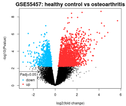 |
A volcano plot displays statistical significance (-log10 P value) versus magnitude of change (log2 fold change) and is useful for visualizing differentially expressed genes. Click the Explore and download link to go to the interactive plot. There, you can mouse-over data points to see individual gene annotation. Highlighted genes are significantly differentially expressed at a default adjusted p-value cutoff of 0.05 (red = upregulated, blue = downregulated). You can change the significance cut-off in the Options tab. A volcano plot displays the test results for a single contrast (a contrast is one Sample group compared to another Sample group). Thus, if you defined more than 2 Sample groups in your analysis, a separate plot is generated for each contrast. By default, for >2 groups of Samples, the number of contrasts presented is equal to the number of groups, and each group is compared to the next in the order that they were created. Alternatively, you can select up to 5 custom contrasts in the Options tab. If more than 2 Sample groups are defined, use the checkboxes to toggle between contrasts. Use the Download significant genes button to download the highlighted genes in each contrast. |
|---|---|---|
| Mean difference (MD) plot | 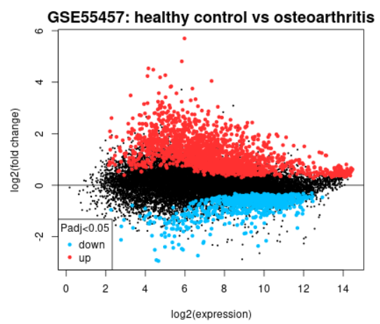 |
A mean difference (MD) plot displays log2 fold change versus average log2 expression values and is useful for visualizing differentially expressed genes. Click the Explore and download link to go to the interactive plot. There, similar to volcano plot, you can mouse-over data points to see individual gene annotation. Highlighted genes are significantly differentially expressed at a default adjusted P-value cutoff of 0.05 (red = upregulated, blue = downregulated). You can change the significance cut-off in the Options tab. A mean difference plot displays the test results for a single contrast (a contrast is one Sample group compared to another Sample group). Thus, if you defined more than 2 Sample groups in your analysis, a separate plot is generated for each contrast. By default, for >2 groups of Samples, the number of contrasts presented is equal to the number of groups, and each group is compared to the next in the order that they were created. Alternatively, you can select up to 5 custom contrasts in the Options tab. If more than 2 Sample groups are defined, use the checkboxes to toggle between contrasts. Use the Download significant genes button to download the highlighted genes in each contrast. |
| UMAP | 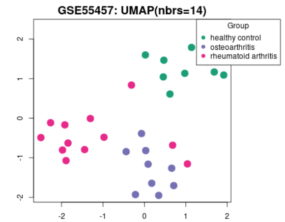 |
Uniform Manifold Approximation and Projection (UMAP) is a dimension reduction technique useful for visualizing how Samples are related to each other. The number of nearest neighbors used in the calculation is indicated in the plot. This plot can be generated without Sample group selection, just click Analyze before defining groups. |
| Venn diagram | 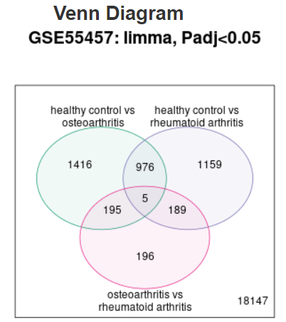 |
Use to explore and download the overlap in significant genes between multiple contrasts.
The genes in each region on the Venn diagram can be downloaded by selecting the relevant
contrasts. For example, in the Venn diagram shown here, select both
'healthy control vs osteoarthritis' and 'healthy control vs rheumatoid arthritis'
to download the 976 significant genes that are common to both contrasts,
but not to 'osteoarthritis vs rheumatoid arthritis'. To download all significant
genes for a given contrast, use the interactive volcano or MD plot pages instead.
Limitation: Data for up to 5 contrasts can be plotted. When >5 groups have been defined, default behavior is to show contrasts with the highest and lowest number of expressed genes. Alternatively, you can select which 5 contrasts to display on the Options tab. |
| Boxplot | 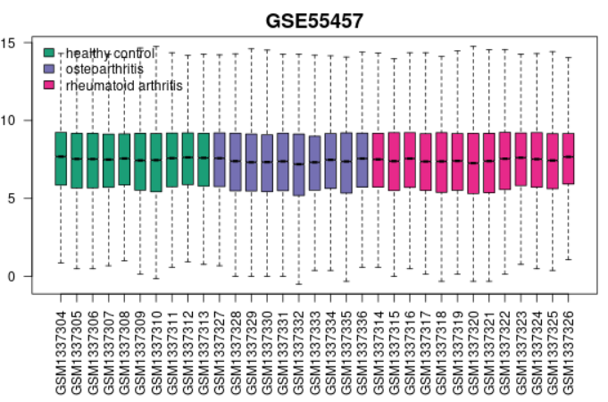 |
Use to view the distribution of the values of the selected Samples. The Samples are colored according to groups. Viewing the distribution can be useful for determining if your selected Samples are suitable for differential expression analysis. Generally, median-centered values are indicative that the data are normalized and cross-comparable. If that is not the case, you might consider checking Force normalization in the Options tab which will apply quantile normalization to the expression data making all selected Samples have identical value distribution. The plot shows data after log transform and normalization, if they were performed. This plot can be generated without Sample group selection, just click Analyze before defining groups. |
| Expression density | 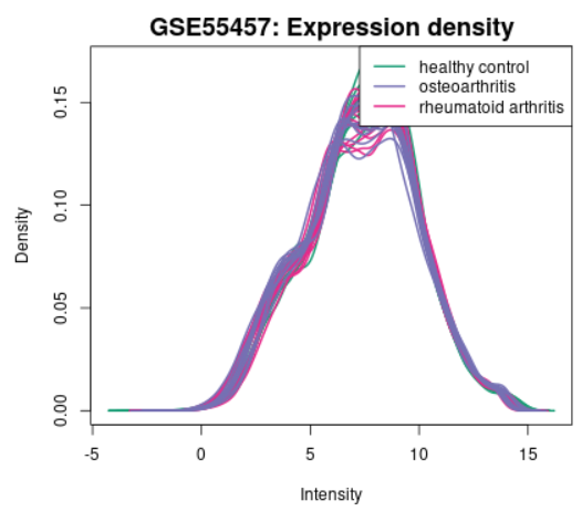 |
Use to view the distribution of the values of the selected Samples. The Samples are colored according to groups. This plot complements boxplot (above) in checking for data normalization before differential expression analysis. If density curves greatly differ from Sample to Sample, you might consider checking Force normalization in the Options tab. The plot shows data after log transform and normalization if they were performed. This plot can be generated without Sample group selection, just click Analyze before defining groups. |
| Adjusted P-value histogram | 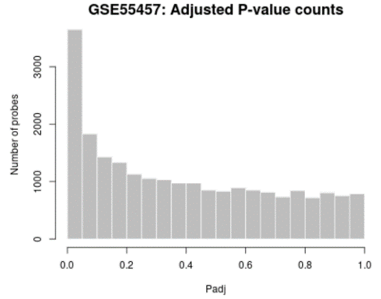 |
Generated using hist
Use to view the distribution of the P-values in the analysis results. The P-value here is the same as in the Top differentially expressed genes table and computed using all selected contrasts. While the displayed table is limited by size (250) this plot allows you to see the 'big picture' by showing the P-value distribution for all analyzed genes. |
| Moderated t-statistic quantile-quantile (q-q) plot | 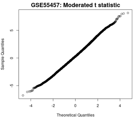 |
Plots the quantiles of a data sample against the theoretical quantiles of a Student's t distribution. This plot helps to assess the quality of the limma test results. Ideally the points should lie along a straight line, meaning that the values for moderated t-statistic computed during the test follow their theoretically predicted distribution. |
| Mean-variance trend | 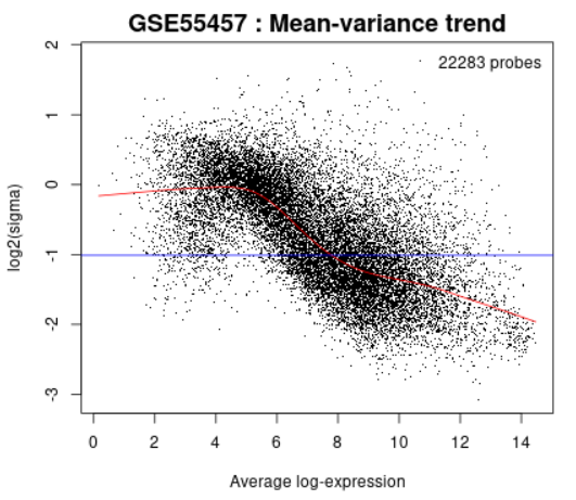 |
This plot is used to check the mean-variance relationship of the expression data, after fitting a linear model. It can help show if there is a lot of variation in the data. This plot can help assess whether applying the precision weights option to take mean-variance trend into account is recommended. Precision weights improve accuracy of test results when a strong mean-variance trend is present. The plot does not require group selection. Each point represents a gene. The red line is mean-variance trend approximation that can be (or already is, if precision weight option in Options tab is checked) taken into account during differential gene expression analysis. The blue line is constant variance approximation. This plot can be generated without Sample group selection, just click Analyze before defining groups. |
Tutorial Video
Edit options and features Back to top
Options
Apply adjustment to the P-values: Limma and DESeq2 provides several P-value adjustment options. These adjustments, also called multiple-testing corrections, attempt to correct for the occurrence of false positive results. The Benjamini & Hochberg false discovery rate method is selected by default because it provides a good balance between discovery of statistically significant genes and limitation of false positives. If you want to change the adjustment method, go to the Options tab and select another method. References for each method are provided below. The adjusted P-values are listed in the Adj P-value column of the results table.
Apply log2 fold change threshold: If you are interested only in genes with larger log2 fold changes you can apply a log2 fold change threshold in the Options tab. The default is set to 0. When you choose a log2 fold change threshold value, only genes with log2 fold change values equal to or greater than the absolute value of the chosen threshold will appear as colored dots in the Volcano, Mean-difference plot and Venn diagram. For example, if you choose a log2 fold change threshold of 3, then only genes with log2 fold change greater than 3 or less than -3 will be colored red or blue, respectively. When a log2 fold change threshold has been chosen in the Options tab, the Download significant genes button will download only those genes that have passed the log2 fold change threshold.
Apply log transformation to the data: (Microarray only) The GEO database accepts a variety of data value types, including logged and unlogged data. Limma expects data values to be in log space. To address this, GEO2R has an auto-detect feature that checks the values of selected Samples and automatically performs a log2 transformation on values determined not to be in log space. Alternatively, the user can select Yes to force log2 transformation, or No to override the auto-detect feature. The auto-detect feature only considers Sample values that have been assigned to a group, and applies the transformation in an all-or-none fashion.
Apply limma precision weights (vooma): (Microarray only) The vooma function estimates the mean-variance relationship and uses this to compute appropriate observational-level weights.
Force normalization: (Microarray only) This function applies quantile normalization to the expression data making all selected Samples have identical value distribution.
Category of Platform annotation to display on results: (Microarray only) Select which category of annotation to display on results. Gene annotations are derived from the corresponding Platform record. Two types of annotation are possible:
NCBI generated annotation is available for many records. These annotations are derived by extracting stable sequence identification information from the Platform and periodically querying against the Entrez Gene database to generate consistent and up-to-date annotation. Gene symbol and Gene title annotations are selected by default. Other categories of NCBI generated annotation include GO terms and chromosomal location information.
Submitter supplied annotation is available for all records. These represent the original Platform annotations provided by the submitter. Note that there is a lot of diversity in the style and content of submitter supplied annotations and they may not have been updated since the time of submission.
Adjusted P-value threshold: Volcano, MA and Venn plots highlight significant differentially expressed genes. The default adj-P-value significance level cut-off is 0.05. You can increase or reduce the significance level cut-off by entering a new number between 0 and 1.
Volcano, MA and Venn contrasts: Volcano and MA plots display data for a single contrast (a contrast is one Sample group compared to another Sample group). Thus, if you defined more than 2 Sample groups in your analysis, a separate plot is generated for each contrast. A maximum of 5 custom contrasts is presented on volcano, MA and Venn plots – for studies with >5 possible contrasts, you can change the contrast selection using the drop-down menu.
Profile graph
This tab allows you to view a specific gene expression profile graph. For RNA-seq data, enter the gene symbol or identifier from the GeneID column of the Human.GRCh38.p13.annot.tsv.gz annotation file. For microarray data, use the identifier from the ID column of the corresponding Platform record. Each red bar in the graph represents the expression measurement extracted from the TPM normalized expression counts (for RNA-seq), or the Value column of the original submitter-supplied Sample record (for microarrays). This feature does not perform any calculations; it merely displays the expression values of the gene across Samples. Sample groups do not need to be defined for this feature to work.
R script
This tab prints the R script used to perform the calculation. This information can be saved and used as a reference for how results were calculated.
Limitations and caveats Back to top
The GEO database is a public repository that archives thousands of original high-throughput functional genomic studies submitted by the scientific community. These studies represent a large diversity of experimental types and designs, and contain data that are processed and normalized using a wide variety of methods. GEO2R can access and analyze almost any GEO Series, regardless of data type and quality, so the user must be aware of the following limitations and caveats.
Results may not match publication: RNA-seq data can be processed using many different software packages, parameter settings and filters and the counts and comparisons generated by the NCBI RNA-seq counts pipeline and GEO2R may not match results in the accompanying publication. The NCBI pipeline represents just one of many possible processing approaches. It is likely the original submitter used different procedures to process their data, which can lead to somewhat different expression results from those generated by the NCBI pipeline.
Missing Samples: Reasons for missing RNA-seq count data include the run didn't pass the 50% alignment rate in the NCBI RNA-seq counts pipeline or processing failed for a technical reason. Reasons for missing microarray values include the submitter was unable to produce data for a given Sample. Regardless of the reason, Samples for which no counts are available are greyed out and can’t be selected for comparison in the Sample table.
Check that Sample values are comparable: GEO submitters often deposit more than one type of sequence data (eg, RNA-seq and RIP-seq) in the same study, meaning that the RNA counts, even within a matrix, are not directly comparable. Other times, although Samples are of the same type, they still may not be intended for comparison. Review the original records to determine if all the Samples within a study are intended to be compared directly. Similarly, for microarray data, GEO2R operates on Series Matrix files which contain data extracted directly from the VALUE column of Sample tables. Submitters are asked to supply normalized data in the VALUE column, rendering the Samples cross-comparable. The majority of GEO microarray data do conform to this rule. GEO applies no further processing other than to perform a log2 transformation on values determined not to be in log space (see Options section). However, some studies, such as dual channel loop design data, may generate values that do not have a common reference and are not directly comparable. Some studies may contain Sample value data that are not normalized, or have a design such that the Samples were never intended to be directly compared. Yet other studies do not have sufficient replicate Samples to perform a robust statistical analysis. Users should examine the original Series to understand the experimental design, and check the 'Data processing' field or VALUE description in the original Sample records for information on what the values represent. Several plots, including boxplot and expression density can be generated without Sample group selection, just click Analyze before defining groups. These plots can help users assess whether the distributions of values across Samples are normalized and cross-comparable.
Data type restriction: (Microarray) GEO2R operates on data in Series Matrix files which contain data extracted directly from the VALUE column of Sample tables. Some categories of GEO Samples do not have data tables (e.g., high-throughput sequencing or genome tiling arrays) and thus cannot be analyzed using GEO2R.
Contrast selection: When more than two Sample groups are defined, GEO2R selects pairwise contrasts in a circular fashion (eg, 1 vs 2; 2 vs 3, 3 vs 4). Thus, the top differentially expressed genes presented in the results table may not fully reflect the user expectation of all possible pairwise contrasts.
Within-Series restriction: GEO2R operates on Series Matrix files. Thus, analyses are restricted to Samples that occur within one Series; it is not possible to perform cross-Series comparisons.
Failed jobs: Occasionally, a GEO2R analysis will fail because some aspect of the input data is not compatible with the GEOquery, limma, or DESeq2 packages. In such cases, native BioConductor errors are reported.
10 minute timeout: GEO2R currently has a 10 minute cutoff imposed on job processing. If the Series you are attempting to analyze has a large number of Samples and/or genes, the analysis may not run to completion.
More information and references Back to top
Summary statistics
RNA-seq:GEO2R provides the following summary statistics as generated by DESeq2. GEO2R uses the Wald test for comparing 2 groups of Samples, and LRT (Likelihood Ratio Test) when comparing 3 or more groups of Samples.
| padj | P-value after adjustment for multiple testing. This column is generally recommended as the primary statistic by which to interpret results. |
|---|---|
| pvalue | Raw P-value. |
| lfcSE | Standard error of the log2FoldChange estimate (only available when two groups of Samples are defined). |
| stat | The Wald statistic (for a two group comparison), or the difference in deviance between the reduced model and the full model (for >2 group comparison). |
| Log2FoldChange | Log2-fold change between two experimental conditions (only available when two groups of Samples are defined). |
| baseMean | The average of the normalized counts taken over all Samples. |
GEO2R provides the following summary statistics as generated by the limma topTable function. More information about each statistic is provided in chapter 10 of the limma users guide.
| adj.P.Val | P-value after adjustment for multiple testing. This column is generally recommended as the primary statistic by which to interpret results. |
|---|---|
| P.Value | Raw P-value. |
| t | Moderated t-statistic (only available when two groups of Samples are defined). |
| B | B-statistic or log-odds that the gene is differentially expressed (only available when two groups of Samples are defined). |
| logFC | Log2-fold change between two experimental conditions (only available when two groups of Samples are defined). |
| F | Moderated F-statistic combines the t-statistics for all the pair-wise comparisons into an overall test of significance for that gene (only available when more than two groups of Samples are defined). |
General references
- Love, M. I., Huber, W., Anders, S. Moderated estimation of fold change and dispersion for RNA-seq data with DESeq2. Genome Biol. 2014;15(12):550.
- Love, M. I., Anders, S., Huber, W. R documentation: Analyzing RNA-seq data with DESeq2.
- Smyth, G. K. (2004). Linear models and empirical Bayes methods for assessing differential expression in microarray experiments. Statistical Applications in Genetics and Molecular Biology, Vol. 3, No. 1, Article 3.
- Smyth, G. K. (2005). Limma: linear models for microarray data. In: Bioinformatics and Computational Biology Solutions using R and Bioconductor, R. Gentleman, V. Carey, S. Dudoit, R. Irizarry, W. Huber (eds.), Springer, New York, pages 397-420.
- Sean Davis and Paul S. Meltzer (2007). GEOquery: a bridge between the Gene Expression Omnibus (GEO) and BioConductor. Bioinformatics 23(14): 1846-1847
- R documentation: Table of Top Genes from Linear Model Fit
Adjustment test references
- R documentation: Adjust P-values for Multiple Comparisons
- Benjamini, Y., and Hochberg, Y. (1995). Controlling the false discovery rate: a practical and powerful approach to multiple testing. Journal of the Royal Statistical Society Series B, 57, 289-300.
- Benjamini, Y., and Yekutieli, D. (2001). The control of the false discovery rate in multiple testing under dependency. Annals of Statistics 29, 1165-1188.
- Holm, S. (1979). A simple sequentially rejective multiple test procedure. Scandinavian Journal of Statistics, 6, 65-70.
- Hommel, G. (1988). A stagewise rejective multiple test procedure based on a modified Bonferroni test. Biometrika, 75, 383-386.
- Hochberg, Y. (1988). A sharper Bonferroni procedure for multiple tests of significance. Biometrika, 75, 800-803.
- Shaffer, J. P. (1995). Multiple hypothesis testing. Annual Review of Psychology, 46, 561-576.
- Sarkar, S. (1998). Some probability inequalities for ordered MTP2 random variables: a proof of Simes conjecture. Annals of Statistics, 26, 494-504.
- Sarkar, S., and Chang, C. K. (1997). Simes' method for multiple hypothesis testing with positively dependent test statistics. Journal of the American Statistical Association, 92, 1601-1608.
- Wright, S. P. (1992). Adjusted P-values for simultaneous inference. Biometrics, 48, 1005-1013.