The public use file (PUF) estimates and the restricted-use file (RUF) estimates were compared in several ways. First, ratios of the PUF estimates and RUF estimates were calculated (similarly, ratios of their standard errors [SEs] were also produced); then correlations between the PUF estimates and RUF estimates and their SEs were produced. Further, overall disclosure treatment effects were evaluated across years by computing global utility measures, such as Hellinger’s distance (HD) and mean relative root mean square error (RRMSE). Finally, trend lines were plotted for a select set of outcome and domain combinations to display a visual snapshot of patterns of PUF estimates and RUF estimates over time.7
4.1. Comparison of Ratios of Estimates and Ratios of Standard Errors
Ratios of estimates and SEs from the PUF data and the RUF data on each substance use and mental health variable were calculated as follows:
where PUF(i) and RUF(i) are the prevalence estimates obtained from the PUF tables and the RUF tables, respectively, and SEPUF(i) and SERUF(i) are their corresponding SEs. Unrounded PUF and RUF estimates were used in the calculation of these ratios, then the ratios were rounded to two decimal places in the tables. Summary statistics of these ratios were calculated, and boxplots were created to view the distributions.
If the ratios of the estimates and the SEs were close to 1, one can say that the PUF provided estimates that were similar to the RUF estimates. For example, the RUF and PUF prevalence estimates of lifetime marijuana use among individuals aged 12 or older in the Hispanic or Latino group in Table SU02.2 in Appendix C were 30.1 and 30.2 percent, respectively, which yielded a ratio of the estimates that was close to 1. The associated SEs of this lifetime substance use measure were 1.03 and 1.05 percent, as produced from the RUF and PUF, respectively, which gave a ratio of the SEs as 1.02. This comparison shows that the 2002 estimates produced from the PUF and RUF for this particular outcome and domain were fairly similar and that there was a 2 percent increase in the SEs produced from the PUF as compared with the SEs produced from the RUF.
Large ratios indicate that the PUF estimates had a larger deviation from the RUF estimates. For example, as shown in Table SU02.8 in Appendix C the prevalence of illicit drug dependence or abuse among persons aged 12 or older who identified themselves as being of two or more races in 2002 was 4.3 and 4.9 percent from the RUF and PUF, respectively, and the SEs were 0.89 and 1.09 percent from the RUF and PUF, respectively. This comparison resulted in a 1.12 ratio of estimates and a 1.23 ratio of SEs, which means that there was a 12 percent increase in the PUF estimate and a 23 percent increase in the PUF SEs.8
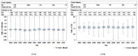
To assess the overall impact of disclosure treatment on NSDUH data quality, the distributions of the ratios of the estimates and the ratios of the SEs were studied to examine the change in precision. Summary statistics for these ratios of estimates and SEs were produced. shows the mean ratios of all of the estimates and the SEs by year for both the substance use measures and the mental health measures for various domain combinations. For the substance use outcomes, each year had about 400 to 600 estimates; for the mental health outcomes, each year had more than 600 estimates. Results show that the average ratios for estimates across years were within the 0.99 to 1.01 range for both the substance use and mental health outcomes; also, the average increase in SEs across years was about 6 to 12 percent for the substance use measures and about 8 to 12 percent for the mental health measures. Note that because each PUF had about a 20 percent reduction in sample size (i.e., the PUF sample size is about 80 percent of the RUF sample size), some increase in SEs for the PUF estimates was to be expected. That is, the ratio of the PUF SEs and the RUF SEs would be roughly around
, which is 1.12; so, the overall PUF estimates were expected to have a 12 percent increase in SEs compared with the RUF estimates. Summary statistics were also run for a set of common tables across years so that roughly similar numbers of estimates (around 400) were evaluated for the substance use measures. The mean ratios of estimates and the mean ratios of SEs were similar to those produced from all of the tables ().
Mean Ratios of Estimates and Standard Errors from the Public Use File Data and the Restricted-Use File Data.
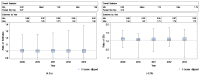
Distributions of the ratios of estimates and SEs from all of the tables are displayed in and for the substance use and mental health outcomes, respectively. These distributions appeared to be stable across years. For the ratios of estimates, data were centered (median) around 1.00, and most estimates had ratios between 0.98 (smallest bottom 25 percent quartile) and 1.02 (largest top 25 percent quartile) for the substance use measures, and 0.98 (smallest bottom 25 percent quartile) and 1.03 (largest top 25 percent quartile) for the mental health measures. Extreme values ranged from 0 to 1.74 and from 0 to 1.38 for the substance use and mental health measures, respectively. For the ratios of SEs for the substance use outcomes, data were centered (median) around 1.07 to 1.12 across years, and most data had ratios between 0.98 (smallest bottom 25 percent quartile) and 1.20 (largest top 25 percent quartile). For the ratios of SEs for the mental health outcomes, data were centered (median) around 1.09 to 1.12 across years, and most data had ratios between 1.01 (smallest bottom 25 percent quartile) and 1.20 (largest top 25 percent quartile). Ratios of SEs spread from 0 to 1.97 and from 0 to 1.79 for the substance use and mental health outcomes, respectively.
Boxplots for Substance Use Measure Comparisons of (4.1a) Estimate Ratios and (4.1b) Standard Error (SE) Ratios.
Boxplots for Mental Health Measure Comparisons of (4.2a) Estimate Ratios and (4.2b) Standard Error (SE) Ratios.
Cases with extreme ratios (i.e., either < 0.5 or > 1.5) of estimates, as well as extreme ratios of SEs, were further evaluated. Among 6,500 estimates (and the corresponding SEs) that were compared for the substance use measures, 43 cases were identified with these extreme ratios. For the approximately 3,400 estimates (and their corresponding SEs) that were compared for the mental health measures, 17 cases were identified with extreme ratios. These extreme cases are shown in (for the substance use outcomes) and (for the mental health outcomes). Relative standard errors (RSEs) for the RUF and PUF estimates were also computed for these cases. Large RUF RSEs means that the estimates were not initially reliable. Cases where the RUF RSE was less than 30 percent were further investigated; of these, 11 out of 43 (26 percent) substance use measures and 7 out of 17 (41 percent) mental health measures had a RUF RSE that was less than 30 percent. For the prevalence measures that demonstrated a substantial difference between the RUF and PUF estimates, formal statistical tests were performed. Not one difference was statistically significant. As indicated in Chapter 2, no formal testing was done except for these handful of cases because it was believed that such tests would be unlikely to detect any significant differences given that the underlying data are almost the same.
Substance Use Outcomes and Domains That Have Extreme Ratios between the Public Use File Estimates and the Restricted-Use File Estimates or Their Standard Errors and Relative Standard Errors.
Mental Health Outcomes and Domains That Have Extreme Ratios between the Public Use File Estimates and the Restricted-Use File Estimates or Their Standard Errors and Relative Standard Errors.
As shown in Table SU09.9 in Appendix C, the 2009 data comparison for past month nonmedical use of pain relievers among past month pain reliever users aged 26 or older who obtained their pain relievers from writing a fake prescription presented a 74 percent higher estimate from the PUF data than from the RUF data, which was the highest ratio of estimates among all of the substance use outcomes. This data comparison also showed a 78 percent increase in SEs from the PUF.
As shown in Table MH13.10 in Appendix D, the 2013 PUF estimate for receiving mental health services in the past year at an inpatient or residential facility among youths aged 12 to 17 who were Asian was 38 percent higher than the estimate from the RUF, which was the highest ratio of estimates among all of the mental health outcomes. This data comparison also had a 68 percent increase in SEs from the PUF.
Patterns were observed where the same measures repeatedly showed extreme ratios across years. For example, both high and ratios appeared in 2009 to 2013 for data comparisons on past month nonmedical use of pain relievers among past month pain reliever users aged 26 or older who obtained their pain relievers from writing a fake prescription (Table SU09.9, Table SU10.9, Table SU12.9, and Table SU13.9). Also, high and low ratios appeared in the 2011 and 2012 mental health tables for data comparisons on receiving mental health services in the past year in juvenile justice settings among youths aged 12 to 17 who belonged to two or more races (Table MH11.11 and Table MH12.11). Each of these extreme ratios can be classified into two categories:
near zero or low prevalence rates, as in the 2004 and 2008 data comparisons on past month OxyContin
® use among individuals aged 12 or older who used alcohol but not cigarettes in the past month (
Table SU04.7 and
Table SU08.7) and the 2013 data comparison on past year crack use among youths aged 12 to 17 with a past year major depressive episode (MDE) (
Table MH13.12); and
small domain or sample sizes, as in the 2007 data comparison on the nonmedical use of pain relievers in the past month among individuals aged 12 or older who were American Indian or Alaska Native (
Table SU07.3) and in the 2013 data comparison on past year illicit drug or alcohol dependence or abuse among adults aged 50 or older who had mild mental illness (
Table MH13.4).
and are color coded to denote patterns in the types of estimates. Estimates with the same color code can be arguably bundled together for outcome-domain combinations, RSEs, small sample sizes, or low prevalence rates.
4.2. Correlations between RUF and PUF Estimates
Estimates from the PUF data and RUF data must be highly correlated as well as their corresponding SEs. To verify this, correlations were calculated between the PUF estimates and the RUF estimates, and correlations were produced among their SEs across years for the selected set of substance use and mental health measures.
indicates that the estimates were highly correlated (as was expected), with correlation coefficients approximately equal to 1.00 for both the substance use and mental health measures. The SEs were also highly correlated, with correlation coefficients between 0.98 and 0.99 for both the substance use and mental health measures.
Correlation of the Public Use File Estimates and Restricted-Use File Estimates and Correlation of Their Corresponding Standard Errors.
4.3. Hellinger’s Distance and Relative Root Mean Square Error
Global utility measures (Dohrmann et al., 2009) were also used for direct assessment or across-year comparisons of disclosure avoidance treatment. Included in this report are HD for tabular counts and RRMSE for point estimates.
HD was calculated as follows:
where RUF(i) = sum of weights for cell i from the RUF tables, and PUF(i) = sum of weights for cell i from the PUF tables. Hellinger’s Distance provides a cumulative measure of how far apart the weighted PUF counts are from the weighted RUF counts for various outcome and domain combinations.
RRMSE quantifies the quality of after-treatment estimates (i.e., the PUF estimates) in terms of both the variation and bias relative to the before-treatment estimates (i.e., the RUF estimates). Thus, the mean RRMSE (M_RRMSE) can be used to assess the treated data quality for estimates from multiple measures:
where Var(PUF(i)) is the PUF sample variance, PUF(i) is the PUF estimate, RUF(i) is the RUF estimate, and m is the total number of estimates.
Equations (3) and (4) were used to obtain the HDs and M_RRMSEs on all of the outcome and domain combinations by year. Because HD is a cumulative measure of PUF counts deviating from the RUF counts, adding more estimates typically results in larger HD values. To compare results across years, the HD was simply normalized by dividing the HD by the square root of the number of estimates to get the normalized HD (). The normalized HDs varied across years and ranged from 10.18 to 15.52 for the substance use outcomes and from 11.74 to 15.40 for the mental health outcomes. HDs assessed for the set of common substance use tables were smaller than the measures for the entire set of tables. However, the normalized HDs from the common tables were roughly similar to the normalized HDs from the entire set of tables.
The M_RRMSE quantifies the bias and variance of the PUF estimates because of the procedures applied for confidentiality protection on the treated data at the global level. On average, the M_RRMSE was fairly consistent from year to year and was no more than 0.13 for both the substance use and mental health measures. The average M_RRMSE was no more than 0.08 for the substance use outcomes based on the common set of tables.
4.4. Trend Comparison
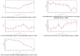
Trend analysis is important in NSDUH for providing information on changes in rates and occurrences of substance use and mental health conditions over time. Such information can be used in substance use, mental illness, and other health condition prediction, prevention, intervention, and new policy development. To examine whether the PUF estimates provide similar trend patterns as the RUF estimates across years, several estimates from the tables that compare the PUF estimates and the RUF estimates were selected. These estimates include, over various demographic domains, mental illness, depression, receiving mental health services, tobacco use, alcohol use, illicit drug use, and receiving drug use treatment. Because the underlying data between the PUF estimates and the RUF estimates were almost the same, no tests of significance between trends were done; however, the trends were assessed by plotting the PUF estimates and the RUF estimates by year to obtain graphical evidence of the overall direction of both trends (i.e., trends from the PUF estimates and trends from the RUF estimates).
The PUF estimates and the RUF estimates over time were plotted to examine whether they provided similar trends. Only a subset of the outcome and domain combinations were selected for plotting, and those plots are displayed in and . For certain measures, the PUF estimates may seem to have varied from the RUF estimates for a specific time point, such as serious mental illness (SMI) in the past year among adults aged 18 or older in 2011. Overall, however, the PUF estimates demonstrated similar trends compared with those from the RUFs. For both the PUF estimates and the RUF estimates, prevalence increased with time (e.g., past month marijuana use among individuals aged 12 or older), prevalence decreased with time (e.g., illicit drug or alcohol dependence or abuse in the past year among individuals aged 12 or older), or oscillations occurred with time (e.g., had at least one MDE in the past year among adults aged 18 or older).
Trend Plots for Substance Use Measures.
Trend Plots for Mental Health Measures.
- 7
For the reader’s convenience, the tables and figures discussed in this chapter are grouped at the end of the chapter so as not to interrupt the discussion. The chapter’s five tables are presented first, then its four figures.
- 8
Individual estimates where ratios were extreme were further examined (see the following discussion).