7.1. Basics and Definitions of Synchrony

Synchrony is a huge topic and the focus of thousands of papers (Pikovsky et al. 2003) covering everything from firefly flashing (Mirollo and Strogatz 1990b) to embryonic development (Ay et al. 2013; Ay et al. 2014). Our goal here is to introduce key ideas in the topic of synchronization, some very recent or novel, which should be widely applicable.

We will illustrate eighteen key properties of synchronization with simple examples. Some hold generally, while others indicate special behaviors that can be seen. We initially consider oscillators of just one variable, and, following the conventions of Winfree and Kuramoto (Kuramoto 1984; Winfree 1967), we denote the number of oscillators as N. As an alternative to the many other reviews of synchronization that focus more on the modeling formalism proposed by Kuramoto (Kuramoto 1984; Pikovsky et al. 2003), we focus mainly on pulse-coupled oscillators. Models that have considered higher-dimensional oscillators, such as the work of Pavlidis (1969), received less attention at first, perhaps because they are more difficult to study. At the end of this chapter, in sections 7.7–7.8, we present recent techniques to study higher-dimensional oscillators.

7.1.1. What Are Coupled Oscillators?

We often assume that each oscillator can easily be identified in the equations and that the coupling can be singled out as well. Sometimes the physiology makes these things clear. For example, individual neurons are often physically distinct, and communication between them is limited to synapses. On the other hand, coupling of biochemical networks remains complex. For example, consider figure 7.1, where two feedback loops share a common element. We may be tempted to consider them one system, but, as the example shown in the figure demonstrates, they can also show properties like those of coupled oscillators.

Figure 7.1

Example of two coupled molecular feedback loops that share the same element, an AB complex. This shared element could also be a signal (e.g., calcium) triggered by both loops. The dynamics of the B loop are much slower than those of the A loop. In this (more...)

Principle of Synchrony 1: Determining individual oscillators from a coupled system can be complex.

7.2. Synchrony in Pulse-Coupled Oscillators

Principle of Synchrony 3: Homogeneous oscillators typically show either phase synchrony or phase desynchrony, perhaps with clusters of oscillators evenly spread over all phases.

We now define the types of oscillators that we will study for most of this chapter. These oscillators are a generalization of the integrate-and-fire model studied in section 6.2. Consider oscillators with phase 0 < ϕ_i ≤ 1 (1 is chosen rather than 2π to match the convention of Mirollo and Strogatz). When ϕ_i = 1, oscillator i “fires” and the phase of each oscillator j other than the firing oscillator is increased from ϕ_j to ϕ_j + p(ϕ_j), which, if >1, causes the other oscillator to fire and synchronize. After firing, an oscillator’s phase is reset to 0 even if other oscillators fire with it. In between firings, all oscillator phases are increased at the same rate until the next firing.

Consider the case of two oscillators. Thinking carefully about these oscillators, one might expect that eventually the oscillator’s phase would be close enough so that when one oscillator fired, the other synchronized. However, another case could occur. Imagine if each time one oscillator fired, the other oscillators had the same phase distribution. This would also be a steady state, and one where the oscillators would never synchronize.

A key question in this field has been to determine when oscillators synchronize and when they do not. Under general conditions, it turns out they will synchronize. To illustrate this process, we include a simulation in figure 7.2. A proof of this fact is offered in section 7.10.

Figure 7.2

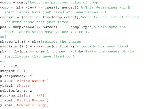
Simulations of 9 coupled oscillations as proposed by Mirollo and Strogatz. The top plot shows the phases of the oscillators (each color-coded) at each firing, and the bottom plot shows how many oscillators fired at each firing. As oscillators synchronize, (more...)

For inhibitory coupling, the opposite occurs. The oscillators typically reach a stable distribution of phases that are spread over all phases. Some may synchronize and form clusters, but they will be clusters firing out of phase with oscillators that are not in the cluster (Golomb et al. 1992). This is illustrated in figure 7.3 and proved in section 7.10.

Figure 7.3

Simulations of 25 coupled oscillations as proposed by Mirollo and Strogatz. The top plot shows the phases of the oscillators (each color-coded) at each firing, and the bottom plot shows how many oscillators fired at each firing. Random initial conditions (more...)

We note that in our earlier example, oscillators fired when they reached a state of phase 1. If this was increased to a larger level (equivalent to increasing the amplitude of oscillators), the coupling signal would be effectively weakened.

Principle of Synchrony 4: The effect of the coupling signal inversely scales with the amplitude of an oscillator.

7.3. Heterogeneous Oscillators

It is the rule rather than the exception for coupled oscillators to be heterogeneous. One possible form of heterogeneity would be for the oscillators to produce coupling signals of different strengths. This turns out not to affect the previous arguments and the proof in 7.10, as we could imagine multiple identical oscillators synchronized with the same phase. These would then fire together, which would be equivalent to one oscillator with a coupling signal strength equal to the sum of those of the individual oscillators. By appropriately increasing the number of oscillators, we could then form an identical problem to that of oscillators with different coupling strengths.

While there are many possible other forms of heterogeneity one can consider, we consider here one of the most common: that the oscillators have different periods but are otherwise identical. If anything, the heterogeneity in period helps them synchronize, in that it can increase the difference between the speeds of the fastest and slowest oscillators, making their phases change more and more likely for a synchronization. In fact, even when uncoupled, heterogeneous oscillators will come arbitrarily close to each other in phase unless their periods are some multiple or fraction of each other’s.

The preceding argument seems to suggest that heterogeneous oscillators are even more likely to synchronize than homogeneous oscillators. However, the opposite is often true, since we do not know if oscillators that are initially synchronized will remain synchronized. After the oscillators are synchronized, they will continue with their own periods until the next pulse-coupled event, and thus desynchronize. So the question we address here is: will heterogeneous oscillators that start synchronized, e.g., because of a synchronizing event, remain synchronized?

This question may initially seem to be a simple function of the coupling strength, and how different the periods are. What matters is the ratio of the difference in period to the coupling strength.

Principle of Synchrony 5: In the limit of strong coupling and small period differences, synchrony can persist. In the limit of weak coupling and large period differences, synchrony will not persist.

An illustration of intermediate coupling is shown in figure 7.4. In fact, in such simulations there may be some oscillators that always remain synchronized and others that always remain desynchronized, even if the oscillators are identical except for their initial states. Such a situation is called a chimera.

Figure 7.4

Intermediate coupling strengths lead to networks that transition into and out of synchrony. This simulation is of 30 coupled oscillators with different frequencies. A denser plot is seen we consider a longer time interval. As can be seen for later firings, (more...)

Principle of Synchrony 6: In between these limits, surprisingly, the question of whether two oscillators stay synchronized depends very much on the state of the other oscillators in the network.

Here is an example:

Consider three oscillators, which all fire together initially. First, consider the case where they are uncoupled. A is the fastest, and when it fires, we denote B’s phase as 1 − ε_B. When B fires, we denote C’s phase as 1 − ε_C. Now if they are coupled, A’s firing could increase C and B’s phase by more than ε_B and B’s firing could increase C’s phase by more than ε_C. In this case, all three oscillators will synchronize once A fires, as this will trigger B to fire, which will trigger C to fire. This is called a cascade, and it helps with synchrony, since the fastest oscillators fire to help the slower oscillators fire. Here B’s firing helps A synchronize with C. If A’s firing would not be enough to bring C to fire since, alone, it would need to increase C’s phase by ε_B + ε_C, the intervention of B would allow them to synchronize.

However, B’s firing can also desynchronize A and C. Consider the case that A and C start synchronized, but have different periods and B is ahead of them so that it will fire before A and C. B will increase both A’s phase and C’s phase. However, since A is faster, and the PRC has a positive slope, it will increase A’s phase more than C’s phase, and make it harder for A to synchronize C. Thus, we see two potentially opposite effects. Previously, we saw that B could help C fire with A, and now B could prevent C from firing with A.

This is a useful place to interject a side note about the cascade to illustrate general principles of coupled oscillations. First, when an oscillator fires in a cascade, it does not affect the oscillators that have just fired. If it did, it would push the phase of the oscillators that have just fired away from those that are about to fire.

Principle of Synchrony 7: Having a refractory period, e.g., having the oscillators insensitive to firing after they have just fired, helps in synchrony.

Next, consider the case where many oscillators in the network are not rhythmic. For example, this may occur if their state approaches some state below the threshold for firing. If they are coupled as part of the network, the coupling can push them over the threshold. This has been explored by many authors (e.g., Enright 1980; Ko et al. 2010; Smolen et al. 1993).

Principle of Synchrony 8: Coupling can cause nonrhythmic oscillators to become rhythmic.

This is illustrated in figure 7.5.

Figure 7.5

Nonrhythmic oscillators can become rhythmic when coupled. This is similar to figure 7.2 with 20 oscillators; however, the last 10 oscillators stop at phase 0.9 before the effects of the coupling are accounted for. All oscillators in the network nonetheless (more...)

There are even examples where no oscillator in the network would be rhythmic when isolated, but the network could become rhythmic when coupled.

In general, intermediate levels of coupling are difficult to study, as there are a potentially infinite number of configurations of the oscillators. However, one key principle holds for most coupled oscillator problems with intermediate levels of coupling:

Principle of Synchrony 9: As more oscillators fire synchronously, they create a larger signal that can synchronize even more oscillators.

This is reminiscent of positive feedback loops, but a better analogy is to phase transitions in physics. Triggering one firing could trigger another, which could trigger another, like a row of dominos falling, except that in the case of dominos, each domino depends only on the previous one, whereas here, each oscillator feels all others.

We now illustrate this key principle. Assume that at least one oscillator has fired, and calculate how many others are brought past threshold to fire. This can be easily seen by considering the cumulative distribution function ϑ(x), defined as

As x goes from 0 to 1, ϑ(x) takes account of the fraction of oscillators in states ranging from 1 down to 0 along the phase coordinate, incorporating into its count those oscillators that are within a distance x of the firing threshold. Note that ϑ(0) > 0, since some oscillator has fired.

Assume that all oscillators with phase 1 − x to 1 have fired. Now we wish to determine if more will fire. The collective signal from these oscillators is εϑ(x)N, where N again is the number of oscillators. More oscillators will be brought to synchrony unless

and this can be visualized by plotting εϑ(x)N and x, similar in spirit to the rate balance plots described in chapter 4, section 4.8 for positive genetic feedback loops. We can also solve εϑ(x)N − x=0 to determine this number.

Note that small changes in ϑ(x) can lead to very large changes in the number of oscillators that synchronize. This makes synchrony very dependent on the initial phase of the oscillators.

This property does not hold for uncoupled oscillators. Uncoupled oscillators ignore each other. There is a slight chance that two of them will have the same phase; however, there is a much lower chance that three uncoupled oscillators will have the same phase, and so on for four, etc. As we have seen earlier, in a coupled case, the states in which just two oscillators have the same phase can be less likely than states in which three or more oscillators have the same phase. Thus, in the coupled case, having more oscillators synchronized increases the likelihood that additional oscillators will join in the synchronization, while in the uncoupled case the opposite happens.

Now consider the case where the oscillators have similar periods, but not quite close enough for all oscillators to synchronize. Again, synchronization events must occur, and these could lead to the network being almost synchronized. However, the coupling is not quite strong enough, and at one point synchronization fails. The key here is that it can fail in an epic way. Imagine that a cascade is happening and one oscillator falls out of place. Now the oscillators that just fired are desynchronized from the oscillators that will next fire in the cascade. This illustrates another key point about intermediate coupling.

Principle of Synchrony 10: For coupling strengths strong enough to cause some synchronization, but not enough to fully synchronize the network, the network can show large changes in the synchrony index over time, alternating between states of near total synchrony and near desynchrony.

This is illustrated in figure 7.4. Such changes in the synchronization of the network are much larger than what one would find occurring in an uncoupled network.

7.4. Subharmonic and Superharmonic Synchrony

Principle of Synchrony 11: Oscillators can synchronize to other oscillators if their periods are approximately related by simple fractions.

This is illustrated in figure 7.6 and discussed by many authors (e.g., Jordan and Smith 1987).

Figure 7.6

Simulations as in figure 7.2, but with 10 oscillators with a frequency of 1 and 10 oscillators with a frequency of 2.1. The oscillators form two populations that synchronize with each other.

Here we consider the synchronization of two oscillators, noting that the same principles apply for larger populations of oscillators. Even if oscillators that start out synchronized do not synchronize at the next firing, a later synchronization could occur. For example, if one oscillator’s period is nearly double the other’s, then the faster oscillator could fire twice, and at its second firing, the firing of the slower oscillator could be close enough for synchronization to occur. Such synchronizations are called subharmonic or superharmonic, coming from the terminology of entrainment (Jordan and Smith 1987): Subharmonic/superharmonic entrainment means that an oscillator synchronizes to a signal that has a longer (shorter) multiple of its own period.

Now consider any two oscillators with different periods. Initially, we regard them as uncoupled. The ratio of their periods can be approximated by

where a and b are integers. Thus, starting with the oscillators synchronized, after a cycles of oscillator A and b cycles of oscillator B (which we denote as a-b synchronization) their phases will again be close, ignoring for the sake of simplicity, the resetting that occurs during the a cycles of oscillator A and b cycles of oscillator B. In fact, for appropriate choices of a and b, we can make this phase difference closer and closer. The strength of the coupling needed to a-b synchronize these two oscillators can be made as small as one would like. By this logic, any two oscillators should eventually synchronize. While this is correct mathematically, experimentally it is not particularly useful, since

1.

the oscillators may synchronize first in a 1–1, 2–1, or some other subharmonic or superharmonic manner on the way to a-b synchronization, and

2.

the amount that the oscillator’s average period will be changed by this a-b synchronization could be minimal, particularly if the ratio of the oscillators’ periods is close to a/b, perhaps even so small that it is impossible to experimentally measure.

7.5. Frontiers: The Counterintuitive Interplay between Noise and Coupling

Intuitively, one would expect that noise internal to oscillators could desynchronize a network, and that coupling would fight against noise, mitigating its effects by averaging over many oscillators (Liu et al. 1997). While noise can desynchronize a network and coupling can overcome noise, these general principles have exceptions that are important to consider.

First, recall that the more oscillators that are synchronized, the stronger the signal to synchronize other oscillators. So while noise may bring some oscillators’ phases apart, it can also bring phases together (Goldobin et al. 2010). If enough phases happen to synchronize, a cascade can synchronize the entire network.

Principle of Synchrony 12: If the effect of the cascade is strong enough, noise can synchronize a network of oscillators. Oscillators can also synchronize to a noisy external signal.

In this section, we therefore consider the same pulse-coupled oscillator model as we discussed previously, however, we change the model to assume that the time needed to go from the reset state to threshold is drawn from a probability distribution. We also study different events that can trigger a cascade, for example, if the first element to fire triggers a cascade, or if it is the third element that does so. Our goal is to determine how accurately the population of oscillators fires.

The standard rule when coupling noisy elements together is that the ensemble noise should decrease by 1/N^1/2 where N is the number of elements (Liu et al. 1997). However, this assumes a simple averaging of the state of the elements, which often does not occur. For example, assume that one oscillator in the network is significantly faster than all the other oscillators. Once this oscillator fires, also assume that the cascade is strong enough to cause all other elements of the network to fire. In this case, the network firing will be just as noisy as the firing of the fastest oscillator.

A slightly less noisy case is where every oscillator has the same average period, but again, it is the first oscillator to fire that synchronizes all the others. As pointed out by Enright (1980), this is much more noisy than, say, having the third-, fourth-, or fifth-firing oscillator, etc., synchronize the network. This property comes simply from probability. The largest variance occurs in the first (or last) element of independent and identically distributed random elements, the next largest variance occurs in the second (or next to last) element, and so on, until the variance of the middle element, with ordinal rank N/2 (or N/2 + 1/2 for N odd), which has the least variance. How a biological oscillator could implement synchronization by these less noisy elements is interesting to ponder: It seems that there would need to be some thresholding with the coupling, and that the effects of the coupling would need to be deferred rather than instantaneous, so that no coupling signal would be sent unless a certain number of oscillators had fired.

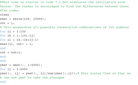
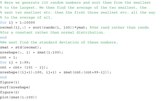
To further test this enhanced noise of the first oscillator to fire, we generate 100 random numbers from a normal distribution 10,000 times, representing 10,000 realizations of the phase of 100 oscillators in a noisy coupled oscillator system (see figure 7.7 and code 7.4). Assume that each oscillator has some large fixed mean period, so that the difference in period between the fastest and slowest oscillator is small with respect to the mean period. We then find the standard deviation of the phase of the oscillator that was the largest of the 100, then the standard deviation of the next largest oscillator out of the 100, and so on, until the smallest. As seen in figure 7.7, top left, the middle oscillators have the lowest standard deviation, suggesting, as before, that these are the least noisy. Now we average the top two phases, then the next two, and so on, until the bottom two, and repeat this for averaging three, four, all the way to a hundred, averaging all the oscillators. This is shown in figure 7.7, top right. Although the average of all the oscillators has the lowest standard deviation, it is not much less than the standard deviation of the middle oscillator. The opposite results are seen for phases taken from a uniform distribution, where the largest or smallest oscillators are the least noisy; see figure 7.7, bottom.

Figure 7.7

Determining the most accurate signal from noisy oscillators. Top left, the standard deviations of 100 Gaussian random variables (representing the phases of oscillators in a noisy system), rank ordered from the largest to the smallest. Top right repeats (more...)

Finally, w noise can cause oscillations in single cells, and coupling can propagate this information to cause an entire network to be rhythmic.

Principle of Synchrony 13: Noise and coupling can synergistically cause rhythms.

However, noise-induced network oscillations can be noisy on the population level, especially if one oscillator could have the effect of triggering a cascade that causes the rest of the network to fire. Ko et al. (2010) present a biological example of this, in which neurons in the SCN are made nonrhythmic by removing the BMAL1 protein. These authors show that rhythms can occur with cooperative effects of noise and coupling. See figure 7.8.

Figure 7.8

Simulations of a network of circadian oscillators. Coupled oscillations occur when BMAL levels are reduced to 10 percent of their original values. At this level, representing the removal of BMAL1, isolated cells are not rhythmic, nor is the network rhythmic (more...)

7.6. Nearest-Neighbor Coupling

Previously, we considered coupling that was all-to-all. When this is not the case, interesting spatial patterns can occur. Although this subject could easily take up a whole book, we will illustrate it with a simple example, inspired by Ermentrout and Kopell (1984), who drew upon work on coupled oscillators in the gut done by several authors (e.g., Linkens 1976). The result we will find here, with oscillators forming clusters with different frequencies, is a special case of the frequency plateaus discussed by Ermentrout and Kopell (1984). We consider a one-dimensional chain of oscillators, while noting that more interesting patterns can occur in two or more dimensions.

Principle of Synchrony 14: Nearest-neighbor coupling can cause spatial patterns.

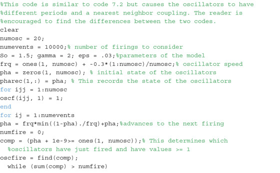
Consider a chain of integrate-and-fire oscillators where each oscillator is coupled only to the previous oscillator. In other words, when one oscillator fires, it affects only the next oscillator in the chain. We also assume that as we proceed down the chain, the frequency of the oscillation decreases. An example of this for 20 oscillators is shown in figure 7.9. The first group of oscillators all fire about 1,300 times. After this, four more pairs of oscillators also fire the same number of times.

Figure 7.9

Simulations with nearest-neighbor coupling. As one proceeds down the chain of oscillators, the autonomous frequency of individual oscillators decreases. See code 7.5 for more details.

This can be understood heuristically by considering the following simple model. Assume oscillators synchronize if their periods have a difference less than ε. In this case, start the oscillators all at a particular phase. When the first oscillator fires, it can cause the next oscillator to fire, and so on. However, when the coupling is not strong enough to bring an oscillator to the same frequency as the first oscillator, that oscillator breaks free. Nevertheless, it can synchronize other oscillators, forming another cluster. An interesting property of this is that it depends on initial conditions. If we now assume the first oscillator does not start with phase zero, it may be the second oscillator that forms the cluster. Such dependence on initial conditions is a property of Turing patterns (Turing 1990), which generate interesting spatial dynamics in coupled oscillators, e.g., the Belousov-Zhabotinskii reaction (Jahnke et al. 1989).

7.7. Frontiers: What Do We Gain by Looking at Limit-Cycle Oscillators?

Consider the case of two coupled van der Pol oscillators. The van der Pol model allows us to explore the effects of having the oscillators described by both phase and amplitude, and having a nonmonotonic PRC as well. This analysis is based largely on course notes by Richard Kronauer (1998), as well as on Rand and Holmes (1980). Here, we adopt one further convention to make clear where assumptions are being made. When an approximation is first made, we indicate it with ≈ but later with = (otherwise most equations would have ≈ and it would be less clear what approximations are being considered).

The specific system we study is

where the oscillators have an uncoupled limit cycle (i.e., a₁₂=a₂₁=0) with amplitude 2. The parameters υ₁ and υ₂ measure the differences between the periods of the oscillators, while ε is a parameter that measures the nonlinearity in the system. The coefficient β determines the relaxation rate to the limit cycle of oscillator 2 in relation to that of oscillator 1, while the cross-coefficients a₁₂ and a₂₁ tell us the strengths of the coupling of oscillator 2 to oscillator 1 and the coupling of oscillator1 to oscillator 2, respectively.

Letting x₁=r₁cos(τ+θ₁) and x₂=r₂cos(τ+θ₂), we convert to polar coordinates. Using the method of averaging, which will be described in detail in chapter 10, one can show that this system is well approximated by

and by letting θ₁₂ = θ₁ − θ₂, we have

Next, let r_i = 2 + δ_i for small δ_i, and i = 1,2 so

and

and we assume that the amplitude of each oscillator quickly reaches equilibrium, so that

which leaves just one differential equation for θ₁₂:

Looking at the fixed points of this equation, one can see that many types of behaviors can occur. First, let (a₁₂ − a₂₁) be large. If υ₁ − υ₂ is small, the oscillators will synchronize 90° out of phase.

Principle of Synchrony 15: The relative coupling strengths can determine the phase difference between the oscillators.

Another case is where a₁₂≈a₂₁. Here, the term (a₁₂ − a₂₁)cos(θ₁₂) disappears, so that is why the last term has been kept. In this case, if υ₁ − υ₂ is small, the oscillators can stably entrain either in phase (0° phase difference) or out of phase (180° phase difference). Also note that, as β decreases, larger values of υ₁−υ₂ can be accommodated.

Principle of Synchrony 16: The smaller the “stiffness” of the oscillator, the larger the range of period differences that can be accommodated.

We calculate the period of the coupled system from

With r₁ ≈ r₂ ≈ 2, we have

So when they are in phase, the frequency is 1 + ε(υ₁ + a₁₂)/2, and it is 1 + ε(υ₁ − a₁₂)/2 when they are out of phase. Thus, the phase configuration can determine the period of coupled oscillators.

More generally, many problems of two coupled oscillators can be reduced to a differential equation for the phase difference between the oscillators (e.g., dθ₁₂/dt), as well as differential equations for the amplitudes of the oscillators. Here, we assumed that the oscillators quickly reached their limit-cycle amplitudes. If we do not assume this, many other behaviors can be seen. One behavior occurs when a stably entrained state loses stability via a Hopf bifurcation (Jordan and Smith 1987). This is known as phase trapping, and it has even been seen in human experimental data (Gleit et al. 2013; Kronauer et al. 1982) (see figure 7.10 for a record of a man living in a cave). In this case, the phase difference between the oscillators (as well as their relative amplitude) oscillates over time with a period that can be significantly different than the period of the oscillators.

Figure 7.10

Human sleep in time isolation. Recorded daily temperature (left) and sleep (right) rhythms from a subject isolated from time cues in a cave. These rhythms are initially in phase, but then exhibit phase trapping (Kronauer et al. 1982). Taken from Chouvet (more...)

Patterns of synchrony can also be found by looking for future times where the system takes the same state, but the state of the oscillators is switched. This we will find in patterns of not only in-phase synchrony but also out-of-phase synchrony. An example of using these techniques to study locomotion is presented by Golubitsky et al. (1999).

7.8. Coupling Damped Oscillators

Here we illustrate a property of coupled limit-cycle oscillators that was recently pointed out by Wang and Slotine (2005).

Principle of Synchrony 17: Damped oscillators easily synchronize.

Consider n oscillators of the form

These oscillators are identical in that they have the same coupling and the same coupled dynamics. Suppose we can rewrite

We then have

This is an interesting form, which all n oscillators then take. While we do not know u_c(z(x₁,…,x_i,…,x_n)), we do know that it is some function of time. Let us define synchrony in the following way. Consider any initial conditions of

and assume that the aforementioned system has a “contracting” property, in that, over time, all initial conditions go to the same value. The system is then no longer a sustained oscillator, perhaps because of the effects of the coupling term, but the system could be a damped oscillator. If this system has the contracting property, the related system

also has this property (and not just for u_c but for any g(t)) (Wang and Slotine 2005). Thus, where we start an oscillator has no bearing on its final state. Since the only difference between the oscillators is their initial state, they must go to the same value and synchronize.

A few words of caution are needed. First, while the preceding argument shows that the different oscillators go to the same state over time, we do not know what this state is. Typically, u_c(z(x₁,…,x_i,…,x_n)) is an oscillation of some sort, but it could also go to a fixed point or show more complex behavior. Second, the argument reduces the coupled oscillator problem to one of different initial conditions of the same system. This may work, but only if the oscillators are homogeneous. Finally, this works typically for larger values of coupling, at least those that can overcome the individual oscillators’ tendency to be sustained and instead contract.

7.9. Amplitude Death and Beyond

An interesting property of coupled limit-cycle oscillators is that when they are strongly coupled out of phase, they can drive each other’s amplitude to zero (Mirollo and Strogatz 1990a). We illustrate this with two coupled van der Pol oscillators. When the oscillators start in phase, oscillations continue. When they start 180° out of phase, rhythms quickly dampen to zero amplitude. See figure 7.11 and code 7.6.

Figure 7.11

Amplitude death. Simulation of two van der Pol oscillators with in-phase coupling (top) and out-of-phase coupling (bottom). In the top, both oscillators start at phase point (1,0), and in the bottom, one oscillator starts at (1,0) and the other at (−1, (more...)

Principle of Synchrony 18: Strongly coupled oscillators can annihilate each other’s amplitude when coupled out of phase.

7.10. Theory: Proof of Synchrony in Homogeneous Oscillators

Here, we present a simple proof of a celebrated result established by Mirollo and Strogatz (1990b) in their work on pulse-coupled oscillators, which answers a question posed by Peskin (1975). In order to preserve the homogeneity of the oscillators, we limit our consideration to cases that have an all-to-all coupling scheme.

We recall the basics of this system described in section 7.2: Consider oscillators with phase 0 < ϕ_i ≤ 1. When ϕ_i = 1, oscillator i “fires” and the phase of each oscillator j other than the firing oscillator is increased from ϕ_j to ϕ_j + p(ϕ_j), which, if >1, causes the other oscillator to fire and synchronize. After firing, an oscillator’s phase is reset to 0 even if other oscillators fire with it. In between firings, all oscillator phases are increased at the same rate until the next firing.

We require that dp/dϕ >0 (and typically assume that p(ϕ) > 0 although this is not required; see the following note), and use ϕ_i^m to denote the state of oscillator i just as the m^th firing occurs. Consider the phase shift to oscillator i caused by the previous N firings, which we will call the “speed” of the oscillator:

Claim: Unless s_r(ϕ_i) = s_r(ϕ_j) for all i, j, a synchronization must occur in finite time.

Note: The requirement that p>0 is not necessary for the proof but does require a different setup to account for the possibility that ϕ + p(ϕ) < 0. To fix this, we require that ϕ + p(ϕ) ≥ 0. This allows for the possibility that ϕ + p(ϕ) = 0, which would mean that, at a firing (when the phase of the firing oscillator goes to zero), another oscillator goes to zero and the two oscillators synchronize in a way similar to the preceding case where one oscillator firing pushes another oscillator above 1.

Proof. Start the oscillators in any configuration, including those that are partially synchronized, and assume that no oscillators will further synchronize. We start our discussion just before a firing occurs. We can find a “fastest” oscillator k so that s_r(ϕ_k) ≥ s_r(ϕ_i) for all i, and a “slowest” oscillator l so that s_r(ϕ_l) ≤ s_r(ϕ_i) for all i, with s_r(ϕ_k) > s_r(ϕ_l). Then, to mod 1, ϕ_k^r−N − ϕ_l^r−N + s_r(ϕ_k) − s_r(ϕ_l) = ϕ_k^r − ϕ_l^r since the only time when the oscillators are advanced at different rates is during a firing. So, over the previous N firings, oscillator k phase-advances with respect to oscillator l by an amount ε = s_r(ϕ_k) − s_r(ϕ_l) mod 1, meaning, for example, if ϕ_k^r > ϕ_l^r, then ϕ_k^r − ϕ_l^r = ϕ_k^r−N − ϕ_l^r−N + ε, or if ϕ_l^r > ϕ_k^r, then ϕ_l^r − ϕ_k^r = ϕ_l^r−N − ϕ_k^r−N − ε. Also, by the definition of s, s_r+1(ϕ_k) − s_r+1(ϕ_l) = s_r(ϕ_k) − s_r(ϕ_l) + p(ϕ_k^r) − p(ϕ_l^r) − p(ϕ_k^r−N) + p(ϕ_l^r−N). Since dp/dϕ > 0, there is a δ such that s_r+1(ϕ_k) − s_r+1(ϕ_l) > s_r(ϕ_k) − s_r(ϕ_l) + δ. In other words, if we consider the state at the next firing (say by oscillator j), oscillator k is phase-advanced with respect to oscillator j when compared to the last time j fired, oscillator l is phase-delayed when compared with the last time j fired, and the difference between the speeds of oscillators k and l, as defined before, also increases.

We can now repeat the argument one firing later, by finding the fastest oscillator and the slowest one. If they are oscillators k and l respectively, the difference between the speed of the fastest and slowest oscillators is s_r+1(ϕ_k) − s_r+1(ϕ_l). If the fastest or slowest oscillator has changed, the difference in speed is greater than this amount. At the next firing, the speed difference must again increase by at least δ. Repeating the argument shows that after each additional firing, the difference in speed between the fastest and slowest oscillators increases again by δ. However, the difference in speed cannot grow arbitrarily large (this would imply, for example, that there is an arbitrarily large phase difference between oscillator k and the other oscillators) without one oscillator overtaking another, an event that would trigger synchronization. QED

This shows that eventually we will end in a state where all the oscillators proceed at the same speed. Does this mean that all initial states will end up synchronized? The answer to this is no. However, Mirollo and Strogatz show that if we pick an initial condition randomly, with probability 1, the end state will eventually be synchronized and not go to one of these states. We can see this based on the following arguments.

Choose a random initial state and encode it as a set of phases (ϕ₁,…, ϕ_N−1) of the N − 1 oscillators when the N^th oscillator has fired. The chance of hitting a partially synchronized state, where two oscillators have the exact same speed, is zero, so we can assume we do not start at a partially synchronized state without any loss. Because of the monotonicity of p, oscillators that have distinct phases before a firing will still have distinct phases after the firing, unless they fire themselves, and this continues to hold for any finite number of firings. Additionally, by the monotonicity of p, oscillators with distinct speeds before the firing, will continue to have distinct speeds. In fact, even stronger properties hold. If we multiply the strength of the firing signal from any oscillator by an integer multiple between 1 and N, they will still have distinct speeds with probability 1. Also, if we remove any number of the oscillators, this would be equivalent to starting with less oscillators, and the oscillators will still have distinct speeds. But synchrony events can be thought of as removing oscillators and multiply the strength of the oscillator they synchronize to by an integer multiple. Thus, with probability 1, another synchrony even will happen, unless all oscillators are synchronized.

For the case of inhibitory firing, we consider the case where dp/dϕ < 0 and we also assume that either d²p/dϕ² > 0 or d²p/dϕ² < 0 (this concave-up or concave-down condition matches many models, including the original by Mirollo and Strogatz, although their example considers dp/dϕ > 0). With these assumptions, the assertion about the oscillators’ behavior is:

Proof: Similar arguments to the preceding proof hold up to noting that there exists δ such that now s_r+1(ϕ_k) − s_r+1(ϕ_l) < s_r(ϕ_k) − s_r(ϕ_l) − δ, and thus the speeds of the oscillators will be brought closer together. The fastest and slowest oscillator speeds will converge until all oscillators have the same speed (note that δ can be bounded from below unless the oscillators have the same speed), which, by the definition of s, means that the oscillators are equidistant from each other. Two possible cases could stop this. First, two oscillators could synchronize, as described before. This will only happen a finite number of times, so each time this happens, we can restart our argument, and the oscillators will again approach the same period. The more difficult case is to determine what happens if after a firing the fastest or slowest oscillator changes.

Consider the fastest oscillator at time r (similar arguments hold for the slowest oscillator). Let it be oscillator k that is the fastest oscillator, a status that we assume switches to oscillator j at the next firing: s_r+1(ϕ_j) > s_r+1(ϕ_k), and before the firing s_r(ϕ_j) < s_r(ϕ_k). This means s_r+1(ϕ_j) − s_r(ϕ_j) > s_r+1(ϕ_k) − s_r(ϕ_k) or p(ϕ_j^r) − p(ϕ_j^r−N) > p(ϕ_k^r) − p(ϕ_k^r−N). We also have ϕ_k^r − ϕ_k^r−N > ϕ_j^r − ϕ_j^r−N, since k was the fastest oscillator, which if d²p/dϕ² > 0 means ϕ_k^r < ϕ_j^r (if d²p/dϕ² < 0, ϕ_k^r > ϕ_j^r). Note that oscillators cannot overtake each other (they can synchronize, which can happen only a finite number of times, we can just start over) so their ordering is fixed. Thus, k cannot later overtake j at a future time, which means that k cannot be faster than j. There are ₂C_N = N!/(2!(N − 2)!) pairings, and only this many possibilities for oscillators to synchronize to each other. QED

Note: One amazing fact is that the preceding proofs also hold for oscillators with different coupling strengths. We can see this by replacing such a network, with a network of oscillators with the same strength, and just add more synchronized oscillators to each phase so that the same overall effect occurs. It also holds when oscillators have different periods. Thus, so long as there is a fastest and a slowest oscillator, there will be another synchrony event in finite time for excitatory coupling. However, the difficulty with period heterogeneity is that after a synchronization, the oscillators may not remain synchronized.

Code 7.1 Two Coupled Biochemical Feedback Loops

.

Code 7.2 Pulse-Coupled Oscillators

(see figure 7.2)

.

.

Code 7.3 Inhibitory Pulse-Coupled Oscillators

(see figure 7.3)

.

Code 7.4 Noisy Coupled Oscillators

(see figure 7.7)

.

.

Code 7.5 Coupled Chain of Oscillators

(see figure 7.9)

.

.

Code 7.6 Amplitude Death

(see figure 7.11)

.

Exercises