Graphical View Legend

This legend applies to NCBI Sequence Viewer. Sequence Viewer can be found embeddedon NCBI pages, as a standalone view, and as the viewer component of the NCBI GDV and Variation Viewer genome browsers.

1. Generic Feature Rendering
2. Gene Model Features
3. Clone Placement Features
4. SNP Features
5. Structural Variants
6. Segmental Duplications
7. Alignments
8. Sequence Track
9. Segment Map
10. Six Frame Translations
11. Label Placement
12. Histogram or Graph Rendering

1. Generic Feature Rendering

This section describes the rendering used for gene features, RNA and protein models, regulatory sites, and most other feature types. These features often derive from files formatted as BED, bigBED, GFF3, GTF, ASN.1, and similar formats.

Specialized rendering for SNPs, structural variants, and segmental duplications are described in the later sections of this documentation.

1.1 Feature Color Code

Feature Type	Color	Visual Examples
Gene	Green
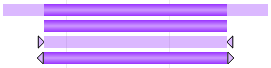
RNA	Purple
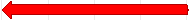
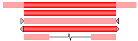
Coding region (CDS)	Red
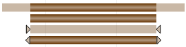
Mature peptide	Golden Brown
Protein feature or other annotated feature	Black
Repeat region	Blue
Regulatory feature	Teal
Protein binding site	Red
Recombination site	Golden Brown
Mobile genetic element	Blue
Miscellaneous feature	Purple

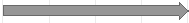
White arrows inside features indicate the direction of the feature relative to the top-level sequence. Grey arrows in introns (e.g. in RNA and coding region features) indicate the direction of splicing.

1.2 Feature Display Options

The track display settings dialog can be accessed by clicking on the track title, the gear icon on the right side of the track, or by selecting the track within the Tracks configuration menu.

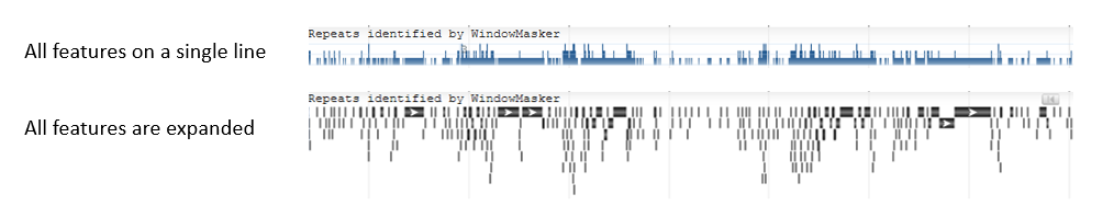
Users can set the display resolution using the Rendering Options dropdown menu. By default, most feature tracks are set to "Pack features if necessary", where individual features are shown when zoomed in and the data is displayed as a histogram when zoomed out. The option "All features on a single line" alway shows the data as a histogram, while the option "All features are expanded" always shows discrete features.

The Feature linking options provide different display views for tracks containing parent and child features; i.e. "Show all"; "Show parent, Merge children"; "Show children, not parent"; "Show parent, not children"; "Superimpose children on parent". Changing these options may result in showing more or fewer features in the track, depending on the underlying source of data in the track.

1.2.1 Intron feature display

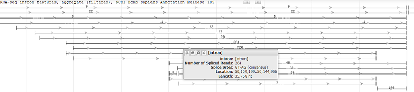
Intron feature tracks display exon-exon splice junctions based on an analysis of RNA-seq data. The ends of the features correspond to splice junctions, while the arrow corresponds to the direction of splicing. The number of RNA-seq reads supporting the splice junction is reported for each feature. Hover over the feature to see a tooltip that provides additional information, including the end coordinates and intron length.

Intron features tracks contain additional track display options, including the ability to sort splice junction features based on the number of spliced reads or by the splice direction (strand). Users can also simplify this track display by filtering the data based on the number of spliced reads.

1.3 Special Rendering Styles

1.3.1 Pseudogene features

Display Settings	Visual Effect	Visual Examples
Show all	Stripes within green gene bar
No gene bar	Green stripe background
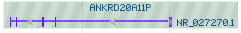
Show on single line with exon structure, no gene bar	Green stripe background

1.3.2 Features with imperfect match to the assembly

Example	Visual Effect	Visual Examples
RNA or CDS feature with sequence discrepancy relative to the assembly	Shaded background

1.3.3 Features with partial annotation location (e.g. due to assembly errors or gaps)

Examples	Visual Effect	Visual Examples
Partial 5’ end	Black arrows ("<<" or ">>") at 5' end
Partial 3’ end	Black arrows ("<<" or ">>") at 3' end
Internal imprecise ends	Black arrows (“<<” and “>>”) at internal junctions
Partial 5’ and 3’ ends	Black arrows ("<<" and ">>") at both ends

1.3.4 Feature marked as partial

Example Cases	Visual Effect	Visual Examples
Feature marked as partial at 5’ and 3’ ends (white arrows, "<<" and ">>") and feature with a partial 3' end (black arrows ">>")	White arrows ("<<" and ">>") at both ends or black arrows (">>") at one end.

1.3.5 Restriction site features

Restriction enzyme recognition sites are rendered with triangle marks indicating the cut sites. Triangle marks are not present at high zoom levels. When the feature is selected using a mouse click, the location of the cut sites is indicated by red hairlines.

View	Visual Effect	Visual Examples
Restriction enzyme recognition site	Triangles indicate cut sites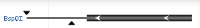
Restriction site (feature selected)	Triangles indicate cut site; hairlines mark feature boundaries and cut sites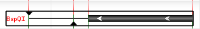
Restriction site (feature selected, zoomed out)	No triangles; hairlines mark feature boundaries and cut sites

1.4 Feature Decorations

Decor Style	Visual Effect	Visual Examples
Default	Solid bars for feature intervals or exons, and solid lines for introns
Arrows	Arrows at both ends showing the strand, and shaded bars for introns
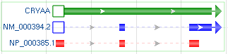
Square Anchor	Square for feature start, arrow for feature stop, dashed lines for introns
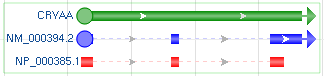
Circle Anchor	Circle for feature start, arrow for feature stop, dashed lines for introns
Fancy	Circle for mRNA start only, square for other features start except for gene and CDS, arrow for feature stop, shaded bars for mRNA introns, and curvy lines for CDS introns

2. Gene Model Features

Gene model features are comprised of multiple possible components: gene bar, RNA/mRNA, CDS, and exon features.

The track display settings dialog can be accessed by clicking on the track title, the gear icon on the right side of the track, or by selecting the track within the Tracks configuration menu. Several options may be available for NCBI or Ensembl gene annotation tracks. The option Hide non-coding will hide non-coding transcripts or non-coding genes or pseudogenes from view, so that only protein-coding transcript variants are displayed. The Hide model transcripts feature hides transcript models predicted using NCBI's Gnomon algorithm.

You may also have options to show only variants that are part of the CCDS project or have been designated as the RefSeq or MANE Select variant.

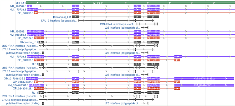
2.1 Gene Model Rendering

Track display settings include multiple rendering options as described below.

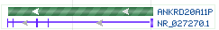
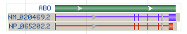
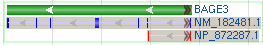
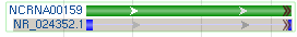
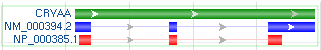
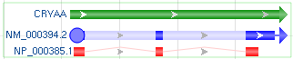
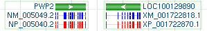
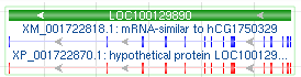
When all features are expanded, gene bars are colored green, non-coding RNAs and mRNA features are colored purple, and CDS features are colored red.

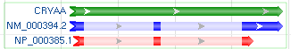
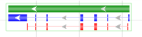
When transcript and CDS pairs are merged, the coding exons are rendered in dark green, and non-coding regions (i.e. 5’ and 3’ UTRs) are rendered in a lighter shade of green, and non-coding RNAs remain purple (See “Merge transcript and CDS pairs, no gene bar” example below).

When all transcripts are merged and merged features include exon portions that are present in some transcripts but missing in other transcripts, the intensity of the green coloring is proportional to the number of transcript variants that include a particular exon region (See “Merge all transcripts and CDSs, no gene bar” example below).

To show features annotated on the RNA or CDS, select the checkbox Show annotated protein features.

Rendering Options	Visual Examples
Show All
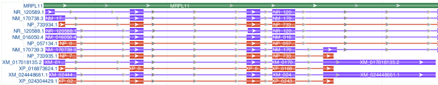
Show all transcripts and CDSs, no gene bar
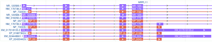
Merge transcript and CDS pairs, no gene bar
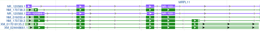
Merge all transcripts and CDSs, no gene bar
Show on single line with exon structure
Gene bar only
Show all, with Product features projected from CDS features

2.2 Special Rendering for discrepancies between RefSeq annotated sequences and genomic sequences

Rendering for mismatches

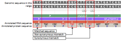
In the case of non-synonymous mismatches, the discrepancy is highlighted by a combination of red colored text for the codon, the display of the alternate bases in the mRNA feature, and the display of the alternate amino acid residue in the protein feature.

In the case of synonymous mismatches, the discrepancy is highlighted by a combination of red colored text for the codon, and the display of the alternate bases in the mRNA feature.

Rendering for insertions and deletions

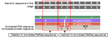
Deletions appear as dash marks in the corresponding mRNA and protein features and lack any display of codons or amino acids.

Insertions appear as a pair of inverted vertical triangles in the mRNA and protein features, and the corresponding codons and amino acids are shown; codons are colored in red.

2.3 Feature Ruler

When all features are expanded in a gene model track, selecting an RNA or CDS feature by clicking on it will reveal a feature ruler indicating the local coordinates of the feature.

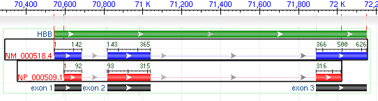
When multiple features are selected, hairlines appear that indicate differences in structure among the different features.

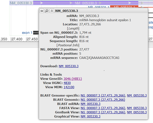
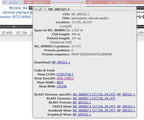
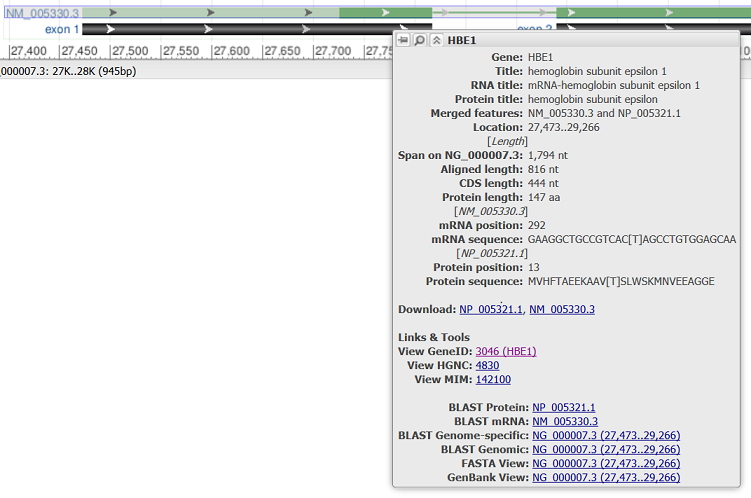
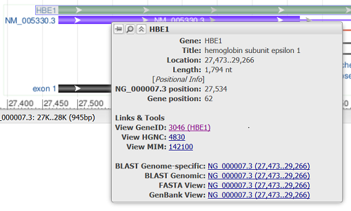
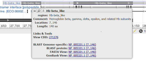
2.4 Feature Tooltip

Hovering over a feature reveals a tooltip with additional information about that feature. The tooltip for gene, RNA, and CDS features reports the feature length, span on the assembly, and the coordinate positions where the tooltip was activated. Links to other NCBI or external resources relating to the gene or feature are also included, where available. There are also options to download the feature in FASTA or GenBank formats, send it to BLAST, or open it in its own instance of the graphical sequence viewer. More information on gene tooltips is available here.

Feature Type	Tooltip Example
RefSeq mRNA
RefSeq CDS
RefSeq merged transcript and CDS
RefSeq gene bar
Projected feature on CDS

3. Clone Placement Features

3.1 Communicated Attributes

Graphical renderings for all clone placement features convey following attributes:

• Concordancy
• Uniqueness
• Clone end confidence
• Directionality, and
• Supporting evidence

3.2 Visual examples for the conveyed attribute

Attribute	Possible Values	Rendering	Visual Example
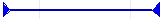
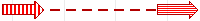
Clone placement type	End-seq only	2 arrows joined by line
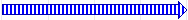
	Insert only	Single arrow
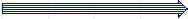
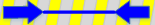
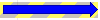
	Combined end-seq and insert	2 arrows joined by line or single arrow on yellow background
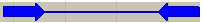
Concordancy	Concordant	Color: Blue
	Discordant	Color: Red
	Concordancy not set	Color: Gray
End-seq only clone placement uniqueness	Unique	Connecting Line: solid
	Multiple	Connecting Line: dotted
	Uniqueness not set	Connecting line: dashed
Clone end confidence	Unique	Fill: solid color
	Multiple	Fill: vertical bars
	Virtual	Fill: empty
	Other/Not set	Fill: horizontal bars
Insert only clone placement uniqueness	Unique	Fill: solid color
	Multiple	Fill: vertical bars
	Other/not set	Fill: horizontal bars
Directionality	Forward or Backward	Arrow
Supporting Evidence	All non-prototype ends are ‘supporting’	With no shaded background
	Not all non-prototype ends are ‘supporting’	With shaded background

3.3 Rendering examples for various attribute combinations

The rendering is able to handle any combination of the five attributes shown above. Below are some rendering examples with various attribute combination.

Display	Description
	Unique, concordant, unique ends
	Multiple, concordant, one unique end, one multiple end
	Uniqueness-not-set, concordant, one multiple end, one confidence-not-set end
	Unique, concordant, one confidence-not-set end, one virtual end
	Unique, discordant, unique ends
	Multiple, discordant, one unique end, one multiple end
	Uniqueness-not-set, discordant, one multiple end, one confidence-not-set end
	Unique, discordant, one confidence-not-set end, one virtual end
	Unique, concordancy not set, unique ends
	Multiple, concordancy not set, one unique end, one multiple end
	Uniqueness-not-set, concordancy not set, one multiple end, one confidence-not-set end
	Unique, concordancy not set, one confidence-not-set end, one virtual end
	Multiple, discordant, one unique end, one multiple end, not all non-prototype ends are ‘supporting’
	Uniqueness-not-set, concordancy not set, one multiple end, one confidence-not-set end, not all non-prototype ends are ‘supporting’
	Unique, concordant, unique ends, not all non-prototype ends are ‘supporting’
	Clone with no end, no strand, unique, concordancy not set
	Clone with no end, plus strand, unique, concordant
	Clone with no end, no strand, multiple, concordancy not set
	Clone with no end, plus strand, discordant, unique not set

4. SNP Features

4.1 Color Code for SNP tracks

This table describes default coloring for SNP features. This coloring applies to dbSNP tracks from the NCBI SNP database and to external/streamed or uploaded VCF files.

See below for details regarding rendering for ClinVar or GWAS tracks.

Variation Type	Color
Single Nucleotide Variation (SNV)	Red
Deletion/Insertion (DELINS)	Blue-Purple
Deletion (DEL)	Blue
Insertion (INS)	Yellow
Multiple Nucleotide Variation (MNV)	Light Gray

4.1.1 Visual Examples

4.1.2 SNP Insertion or deletion

Additional notation distinguishes insertions and deletions.

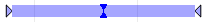
Insertions are marked with two hourglass-like triangles:

Deletions are marked with a triangle pointing downwards:

4.2 Rendering for ClinVar tracks

VCF data tracks from the NCBI ClinVar project have distinct coloring and rendering.

ClinVar Interpretation	Color
Pathogenic; Established risk allele	Dark magenta
Likely Pathogenic; Likely risk allele	Pink
Benign	Dark Green
Likely Benign	Green
Drug Response	Blue
Not provided; Uncertain significance; all other ClinVar statuses	Dark Gray

The track labels indicate the ClinVar variation accession and the ClinVar allele.

Additional information, including the ClinVar review status and the predicted molecular consequence, can be found in the feature tooltips.

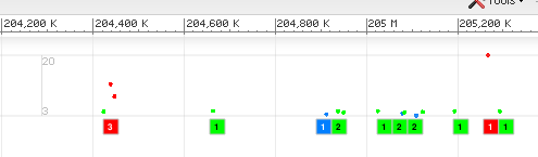
4.3 Rendering for Genome Wide Association Results

This section describes rendering for genome-wide association study (GWAS) analysis from NCBI dbGaP.

The color represents the highest p-value in that bin.

p-Value Range	Color
< 2	Teal
2-3	Sky Blue
3-4	Blue
4-5	Green
5-6	Yellow
6-7	Orange
> 7	Red

The scatter plot above the bins reflects individual p-Values. Both the color (which uses the same coloring scheme) and the dot's location on the Y axis correspond to the p-Value.

5. Structural Variants

This section describes rendering for structural variants with NCBI dbVar identifiers.

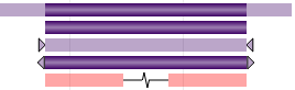
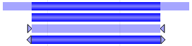
5.1 Common Rendering

There are four common scenarios for most variants (either SVs or SSVs) as shown in the table below. However, mixed cases with a defined breakpoint at one end and an undefined breakpoint range at the other end are possible as well. Here, we use (CNV SV) as examples:

Breakpoint Type	Rendering	Visual Example
With breakpoint resolution	Fully saturated color
With defined breakpoint range	Transparent color for breakpoint ranges
With undefined breakpoint, but known outer bound	Triangles pointing toward each other
With undefined breakpoint, but known inner bound	Triangles pointing away from each other

5.2 Variant Call Types (SSV) and Region Types (SV)

Type	Comment	Visual Example
Copy number variation	Color: violet Four common cases, plus CNV with length of deletion (CNV)
Copy number gain or Duplication	Color: blue (Gain SSV)
Copy number loss or Deletion	Color: red The last one is a loss variant with length of deletion (Loss SSV)
Mobile element insertion or Novel sequence insertion	Color: blue (Insertion SV or SSV)
Tandem duplication	Color: deep brown (Eversion SV or SSV)
Inversion	Color: light violet (Inversion SV or SSV)
Translocation	Color: light indigo with pattern (Translocation SV or SSV)
Complex	Color: light azure (Complex SSV)
Insertion/Deletion or Indel	Color: red
Unknown	Color: grey (Unknown SV or SSV)

Note:

1. SV region type “Copy number variation” can only have children of SSV Types “Copy number gain” and/or “Copy number loss” - in any combination. If all child SSV of a given SV are copy number gain or copy number loss, then the SV will be colored with the same way as the children are colored, blue for gain and red for loss, respectively. If the children are a mix of these two types, then the SV will be colored as violet.

2. SV Type “Complex” can have either:

3. children all of SSV Type “Complex,” or

4. children of two or more SSV Types, in any combination (except “Copy number gain” and “Copy number loss,” which are covered above)

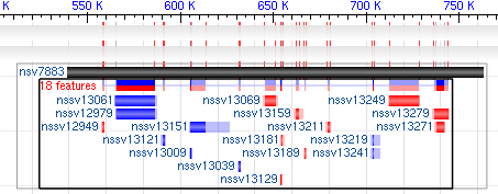
5.3. Rendering Styles for Linked Structural Variants Group

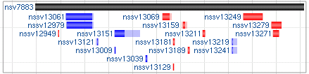
5.3.1 Default rendering with both parent and children shown

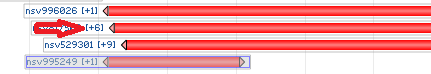
5.3.2 Rendering with supporting variants in a packed form

If there are multiple types in the supporting variants, multiple colors will be used to reflect the corresponding allele type.

Click and select the packed feature bar to show all the supporting variants.

5.3.3 Superimpose all supporting variants over the parent variant

The supporting variants are superimposed on top of the parent variant with the shortest variants on the top. The colors reflect the corresponding allele type.

Click and select the packed feature bar to show all variants.

5.4. Interactive Visualization of Variant Region Child Calls

Set Rendering options of the variation tab of the Configure dialog as "Show parent, Expand children upon a click".

Sequence Viewer will show a plus sign with the number of child tracks for each parent track.

Click on the plus sign, and Sequence Viewer will show all the child tracks and display the minus sign instead of plus at the parent track.

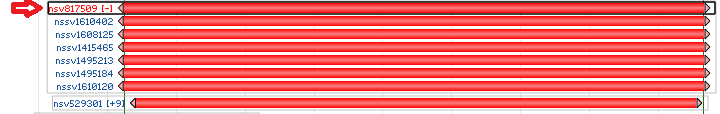
Click on the minus sign to collapse the child tracks again.

6. Segmental Duplications

Identity Attribute	Color	Example
> 99.0	Orange
> 98.0	Yellow
> 90.0	Grey
<= 90.0	Black

7. Alignments

Alignment tracks contain discrete sequences aligned pair-wise to the top-level assembly. These tracks are derived from sequence alignments reported in BAM or similar formats. Assembly-assembly alignments and NCBI BLAST results are also visualized as alignment tracks in the graphical sequence view.

7.1 Alignment Display

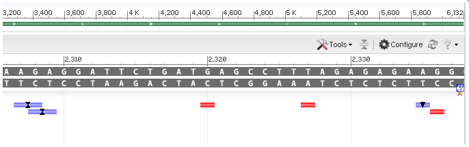
When the Alignment Display is set to “Adaptive” (default), alignment data is represented differently at different zoom levels (Figure 7.1.1). The Alignment Display can also be set to “Packed” (always shows the coverage or pile-up view), “Ladder” (one alignment per row) and “Show all” (always shows individual alignments). These options are found in the track display settings menu (Figure 7.3.1 and Table 7.3).

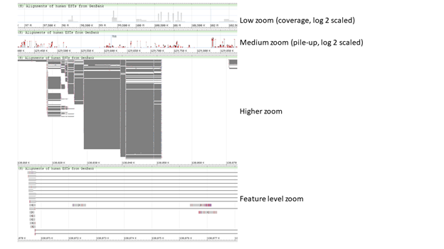
Figure 7.1.1. View of alignments at different zoom levels when Alignment Display is set to “Adaptive”. At lower zoom levels, the alignments appear as a coverage or pile-up graphs in log 2 scale. At higher zoom levels, individual alignments become visible. Note that gaps and mismatches are colored in red.

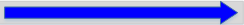
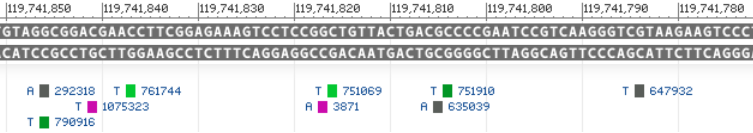
At high zoom levels, alignment details become apparent. By default, matched bases and introns are colored in grey, mismatches and gaps are colored in red, and insertions are represented by blue bars (at higher zoom levels) or a blue hourglass with vertical blue bars proportional to the number of inserted bases (Figure 7.1.2). Less-than or greater-than signs (< or >) indicate the orientation of the alignment relative to the assembly.

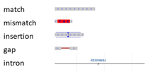
Figure 7.1.2. Legend of alignment features.

7.2 Alignment Tooltips

Hovering the cursor over a discrete alignment reveals a tooltip that lists additional information about the alignment (Figure 7.2.1). Tooltips report the coverage, identity, and number of mismatches, introns, unaligned regions, and gaps in the alignment. The coverage is calculated as the number of aligned bases divided by the total length of the feature sequence, while the identity is calculated as the number of matched bases divided by the aligned length (excluding gaps or introns, with no gap penalty).

If available/applicable, the CIGAR string is also provided. There is also a link to the sequence FASTA of the original aligned feature. In addition, unaligned 5' and 3' nucleotides are indicated at the bottom of the tooltip and can be viewed by pressing the View button.

When the tooltip is generated at or next to the position of an insertion(s) in the alignment, information about the insertion is reported in the Unaligned Regions section of the tooltip. All coordinates are reported relative to the aligned feature. Up to three insertions are reported in a single tooltip.

The tooltip can be "pinned" using the pushpin on the top left. All information provided in the tooltip can be highlighted and copied to the clipboard. Clicking on the magnifying glass on the top resets the graphical view around the selected feature.

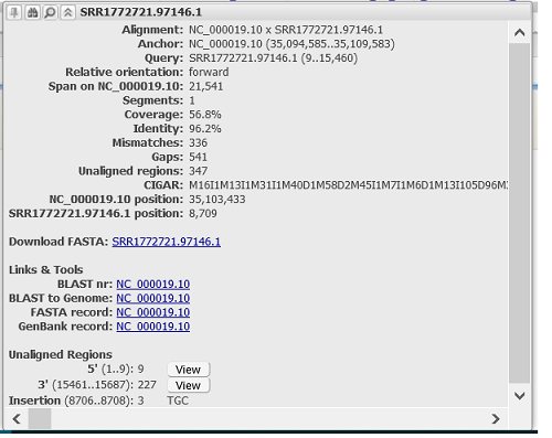
Figure 7.2.1. Tooltip for an alignment feature reporting coverage, identity, and number of mismatches, gaps, and unaligned regions in the alignment. Sequence and coordinates for Unaligned Regions is available at the bottom of the tooltip. Information for insertion(s) is provided if the tooltip is generated at the position of an insertion.

7.3 Alignment Display Options

The track display settings can be accessed by clicking on the track title or selecting the Configure Tracks option under the Tracks button on the toolbar. The track display settings menu (Figure 7.3.1) for alignment tracks provides a variety of different display and analysis options (Table 7.3). These options may include creating a pile-up view, projecting features (Figure 7.3.5), and linking mate pairs (Figure 7.3.6). When the Show pileup option is selected, a pile-up view appears above the alignment (Figure 7.3.2). The Pileup Display dropdown menu includes options for the pile-up, including showing a match/mismatch graph (default view, Figure 7.3.2), match/mismatch table (Figure 7.3.3), or ATGC table (Figure 7.3.4). The Unaligned Tails dropdown menu includes options to show/hide unaligned tail lengths and unaligned sequences. For tracks where the metadata is available, users can also hide alignments (duplicates, bad reads) (Figure 7.3.7) or sort alignments by strand or haplotype.

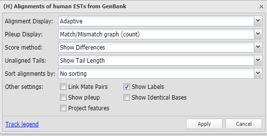
Figure 7.3.1. Track display settings for alignment tracks.

Additional display options are available for Assembly-assembly alignment tracks provided by NCBI. These tracks are comprised of first-pass and second-pass alignments, all of which will be shown by default in the view. First-pass alignments are sequences that have their reciprocal best alignment on both assemblies (reciprocity score 3). Second-pass alignments have a better alignment on one of the assemblies at another location (reciprocity score 1 or 2). The Sort Alignments dropdown menu for Assembly-assembly alignment tracks contains an additional option to sort the view of the track by reciprocity score (first-pass versus second-pass). Second-pass alignments can also be hidden from view by clicking off the check box Show second-pass alignments (checked on by default). The reciprocity score for Assembly-assembly alignment tracks is also reported in the tooltips of individual alignments.

Display Category	Dropdown Menu Options
Alignment Display	Adaptive Packed Ladder (one alignment per row) Show all
Pileup Display	Match/Mismatch graph (count) Match/Mismatch graph (percentage) ATGC graph (count) ATGC graph (percentage) Match/Mismatch table (count) Match/Mismatch table (percentage) ATGC table (count) ATGC table (percentage)
Score method*	Column Quality score DNA Frequency-Based Difference Show Differences Nucleic Acid Colors Quality Score Disabled
Unaligned Tails	Hide Show Tail Length Show Sequence
Hide alignments*	None Duplicates Bad reads Duplicates/Bad reads
Sort alignments by*	No sorting Alignment strand Haplotype Reciprocity score

Table 7.3. Alignment display options found in dropdown menus in the track display settings menu. *These options may not be comprehensive and may differ depending on the nature of the underlying track data.

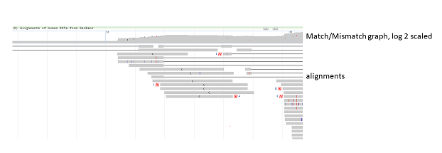
Figure 7.3.2. When the Pileup Display is set to “Match/Mismatch graph” (default), a pile-up graph displays above the alignments. Red markings in the graph denote mismatches while black markings denote gaps. Alignment display in figure is truncated.

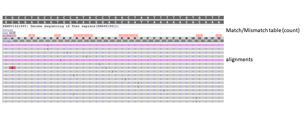
Figure 7.3.3. When the Pileup Display is set to “Match/Mismatch table (count)”, a pile-up table displays above the alignments. When zoom is set to sequence level, counts for intron, gap, mismatch, match, and total are reported for each position. A blank entry denotes a count of 0. Alignment display in figure is truncated.

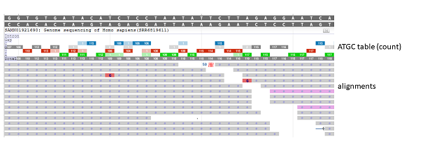
Figure 7.3.4. When the Pileup Display is set to “ATGC table (count)”, a pile-up table displays above the alignments. When zoom is set to sequence level, counts for total, A, T, G, C, gap, and intron are reported for each position. Each nucleotide is represented by a different color; the intensity of the color is correlated to the proportion of matches to that nucleotide at that position. A blank entry denotes a count of 0. Alignment display in figure is truncated.

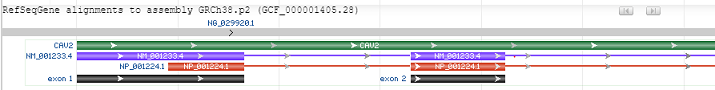
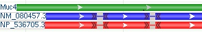
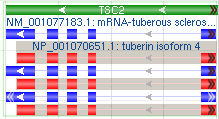
Figure 7.3.5. A RefSeqGene alignment feature (NG_029920.1) with the Project features option selected shows annotated RefSeq transcript (NM_), protein (NP_), and other features.

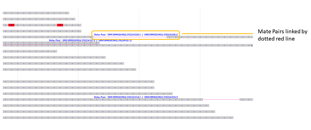
Figure 7.3.6. When the Link Mate Pairs option is selected, sequence mate pairs, if indicated by the metadata in the track, are linked by a dotted red line in the alignment display. When the Show Labels option is selected, labels for mate pairs are displayed.

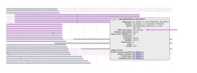
Figure 7.3.7. PCR duplicates, if indicated by the metadata in the track, are colored in purple. PCR duplicates may also be reported in the feature tooltip. Duplicate alignments can be hidden from view by choosing “Duplicates” under the Hide alignments dropdown menu.

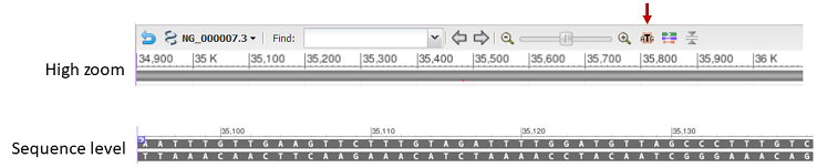
8. Sequence Track

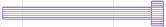
The sequence track is represented by a solid bar at high zoom levels. Clicking on the zoom to sequence button (indicated by arrow below) changes the zoom level to show the sequence.

For nucleotide sequences, both the primary and complementary strands are shown. 5’ marks (circled in blue) at each end of the track indicate the strand orientation.

By default, the sequence track is located just below the ruler and the track label is hidden. The position of the track can be changed via drag and drop.

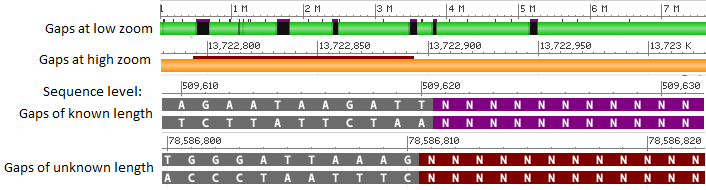
The track display setting for the sequence track is accessible in the track configuration panel and provides the option to show the label for this track and color gaps by gap type.

If the Color gaps by type checkbox is selected, the gaps will be colored according to the annotation in the corresponding INSDC access for the sequence (i.e. annotation in the GenBank flat file record). Gaps of known length will be colored purple, gaps of unknown length will be colored reddish brown, and contaminants will be colored yellow. The color will appear as an extra line above the sequence track at low/high zoom levels and as a background color at the sequence level.

8.1 Segment Color Code

For assembled sequences (e.g. genome assemblies), different types of sequence segments will be colored differently depending on the nature of the underlying component.

Segment Type	Finished HTGS	Draft HTGS	WGS	Other	Gap
Color	Blue	Orange	Green	Grey	Black
Visual example with underlying components

The Gap segment may be colored other than Black when Color gaps by type is checked (see above).

8.2 Restriction site map

Restriction enzyme recognition maps, for instance MAP_000012.1, can be viewed as sequence tracks with the restriction sites indicated by green triangles below the sequence bar.

View	Visual Example
Zoomed-out view
Zoomed-in view with tooltip popped up (if mouse hovering over the site)

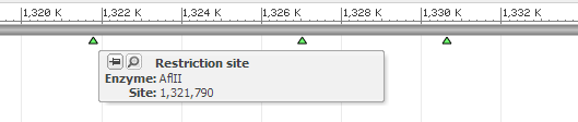
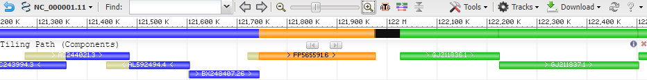
9. Segment Map

Scaffolds (contigs) and tiling path (components) data tracks can be found under the Sequence vertical tab group in the track configuration panel.

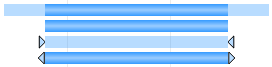
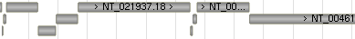
9.1 Scaffolds

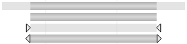
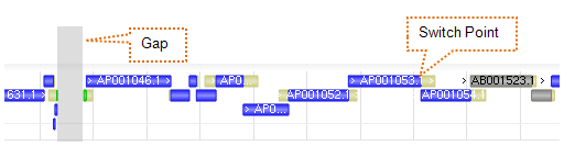
9.2 Tiling Path (Components)

Coloring of tiling path features follows the color scheme in Section 8.1. Overlapping regions not in the path are colored in yellow.

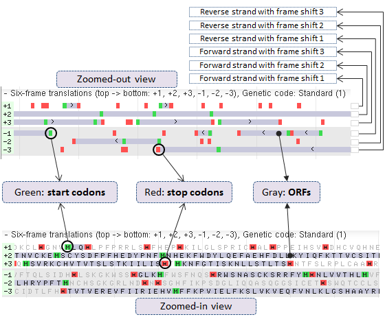
10. Six Frame Translations

11. Label Placement

There are four global options regarding label placement: default, side label, top label, and no label. "Default" may mean different settings for different objects. For example, default label placement for alignments is top labeling, but default setting for features is side labeling.

11.1 Side Label vs. Strand

In side labeling mode, the label is always placed at object's 5' side.

11.2 Examples

Label Placement	Visual Example
Default	Alignment (top):
	Component (inside):
	Features (side):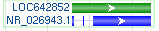
Side Label
Top Label
No Label

12. Histogram or Graph Rendering

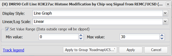
Histogram or graph representation is used to visualize data that are distributed as data counts per position. This data is often in Wig, bigWig, or bedGraph format. Data types displayed as graphs include RNA-seq, epigenomic, and conservation data. Track display settings allow users to choose among display styles ("Histogram", "Heat Map", "Line Graph") and scale ("Linear", "Log Base 10", "Log Base e", "Log Base 2").

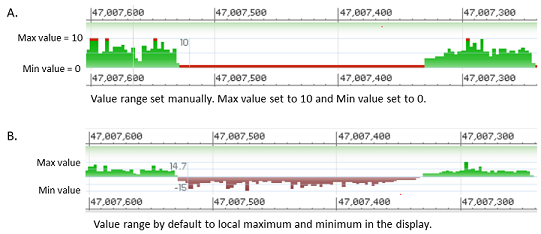
By default, the value range of a histogram or line graph follows the local visible minimum and maximum values in the display. Zooming, panning, or otherwise changing the displayed region will cause the minimum and maximum values to adjust accordingly.

The user may select the Set Value Range option to manually control the value range in the display. This option is available when the display style is set to "Histogram" or "Line Graph" and the scale is set to "Linear". If the data provider has stipulated minimum and maximum values for the track, the Min value and Max value fields will be pre-populated with these values. The user can apply pre-populated value ranges or customize the value range manually. If the track is part of a composite track group from a track hub, the option is available to apply the settings in bulk to all displayed tracks in the composite group.

Upon applying custom minimum and maximum values, any graph data that exceeds a set value range will be clipped in the display and colored in red to alert the user. When the Set Value Range option is deselected, the value range will revert to use of the local minimum and maximum in the display.

12.1 Track Hubs: multiWig Tracks

Some track hubs include multiWig files, which are comprised of multiple subtracks. MultiWig files are shown in the graphical display as merged graphs with each subtrack in a different color (Figure 12.1.1). The track display settings for multiWig tracks provides options to adjust the scale and to display subtracks in a stacked versus merged format.

Clicking on the subtrack legend reveals a subtrack display settings dialog (Figure 12.1.2). Users can adjust the color, opacity, and display style of individual subtracks, which are listed in a drop-down menu. There is also an option to hide individual subtracks.

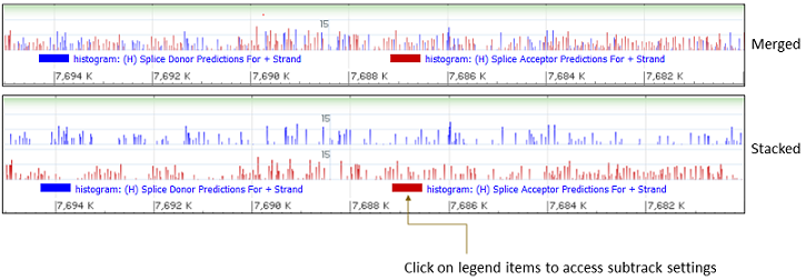
Figure 12.1.1. Merged versus Stacked views of multiWig files. Click on the legend to access subtrack display settings.

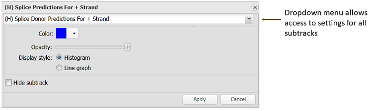
Figure 12.1.2. Subtrack display settings dialog. The dropdown menu provides access to settings for all subtracks within the multiWig track.